Drill: Financial Report

Overview

For this drill example you will use the PL Trend report that was previously featured in the Financial Report - Walkthrough. For this example, you will set up a ReportDrill function to drill to a separate workbook. This can be very useful when there is a common report, such as one that shows general ledger detail, that can be used as a drill from several different reports and workbooks. You will be viewing that same example with the JE (Journal Entry) Query drill report.

If you are following the Training Labs, this report file can be found in the Report Library at Training Labs > Lab 4 Drilling To Data > Lab 4.3 Financial Report.

Opening the Report

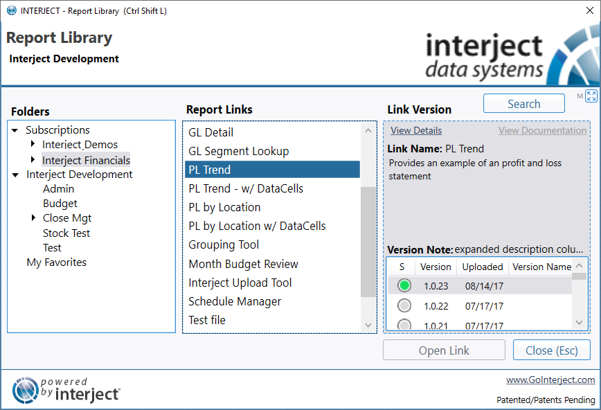
For this example you will be using the PL trend report found in the Interject Financials subscriptions.

Unfreezing the Report

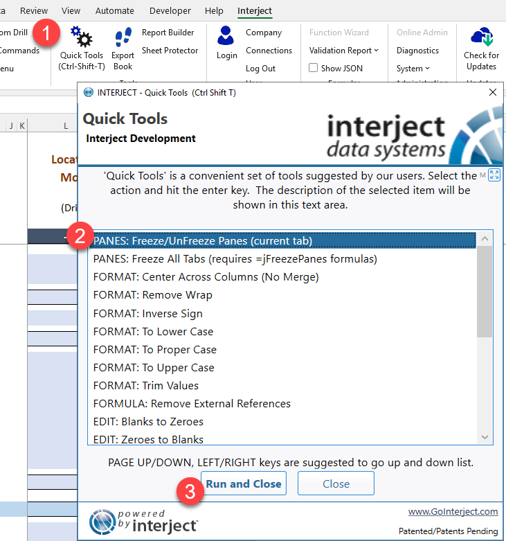
To unfreeze the panels, click on Quick Tools from the Interject tab. Then select PANES: Freeze/Unfreeze Panes and click Run and Close.

Set Up the Report

If you scroll up, you will find that there are already drills set up in this report.

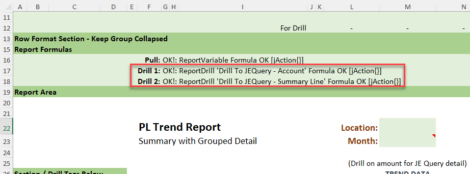
You will delete these drills in order to gain the experience of setting this drill up manually.

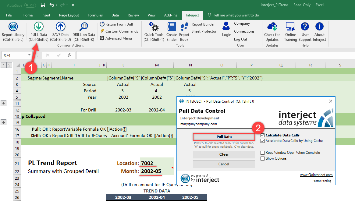
Clear the drills and delete row 18.

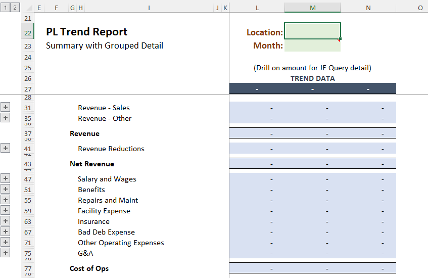
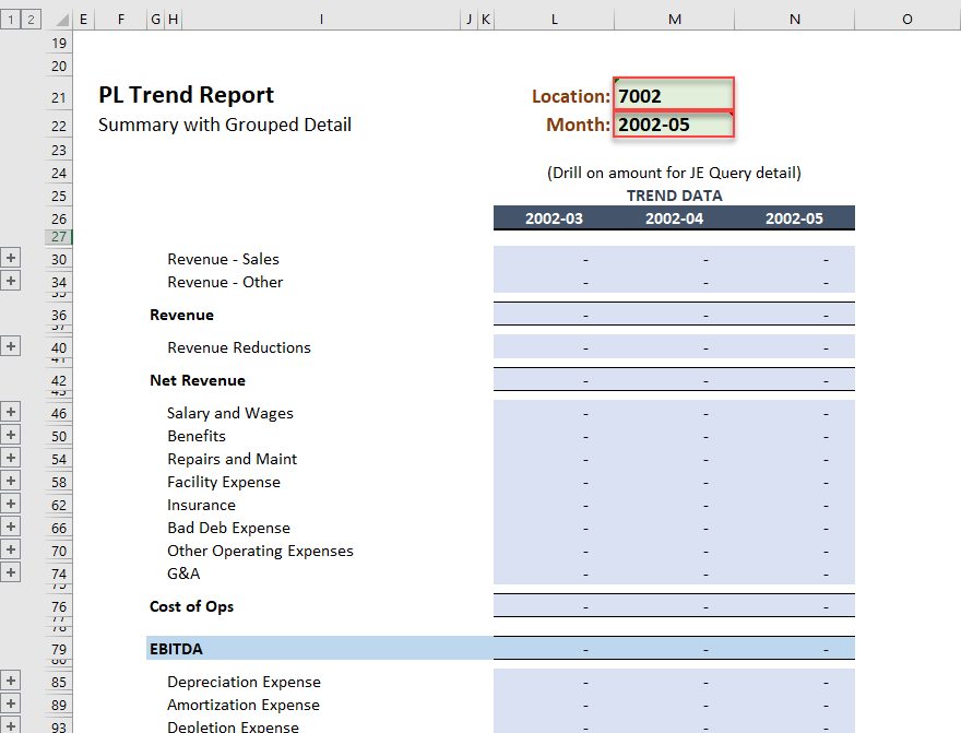
Next, type in 7002 for the location in M21. And type 2002-05 for the month in cell M22.

Building the Drill

Now you will begin to set up the drill.

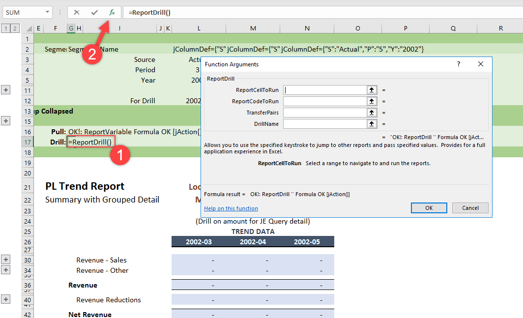
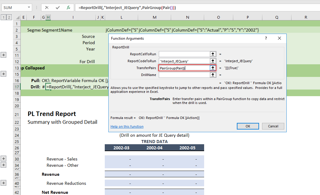
Step 1: In cell G17, type =ReportDrill(). Column G is fairly narrow, but it will simply overlap the cells to the right. Then click the fx button as illustrated below to bring up the Function Wizard.

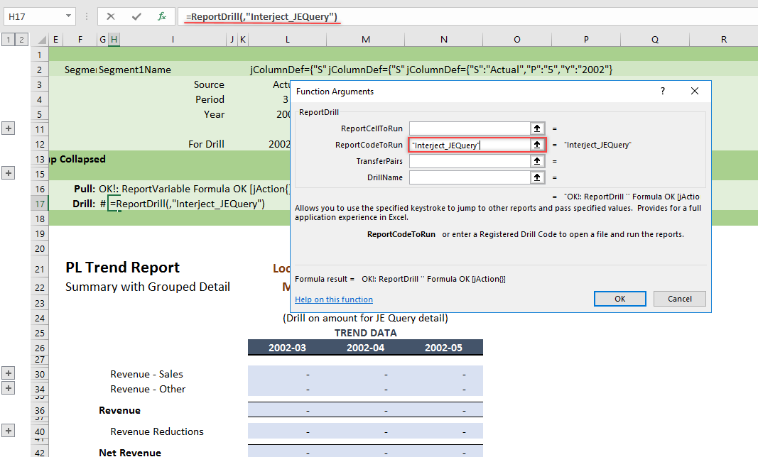
Step 2: In previous drill exercises you have used the ReportCellToRun argument. That is only for drilling within the same workbook. In this example you are drilling to a separate workbook. Type Interject_JEQuery into the ReportCodeToRun argument as seen below. Interject uses drill codes to run drills in a separate workbook. For convenience, this drill code has already been set up in the Report Library report. You will learn how to setup a Drill Code in the next drill exercise.

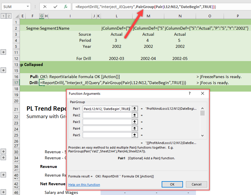
Step 3: Next you will use the TransferPairs argument to note which cell values in the source worksheet will be transferred to the target worksheet during the drill operation. To do this, use special functions to pair the source cells to the target cells. Type PairGroup(Pair()) in the TransferPairs argument to get it started. You will return to add more to this argument.

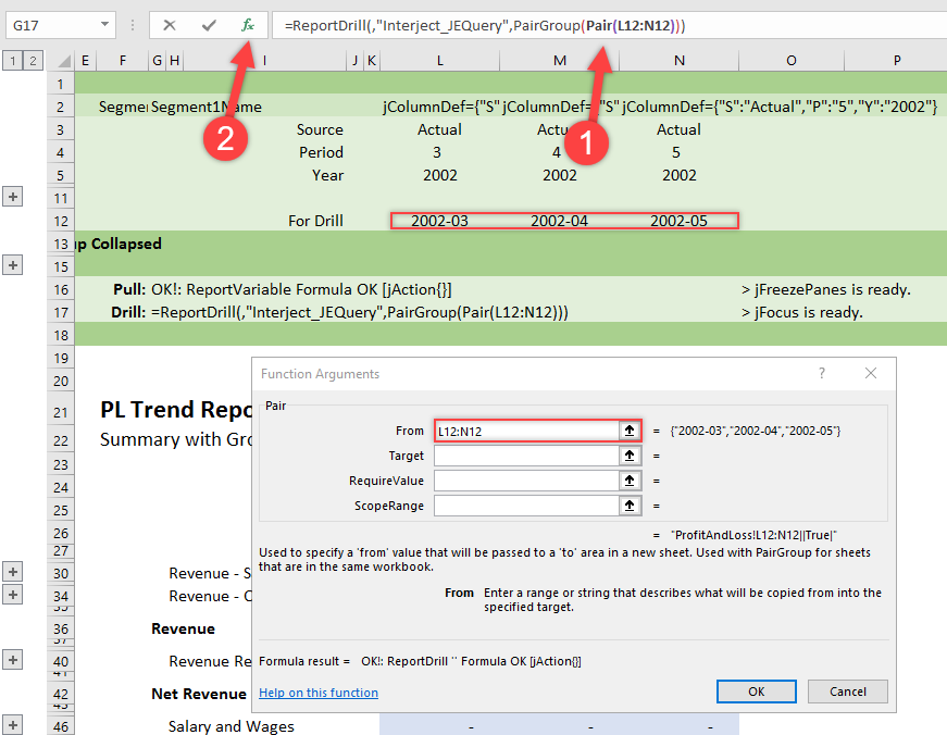
Step 4: In the Formula Bar, click within the word Pair() inside the text PairGroup(Pair()) . See the illustration below. Once this is done, the Function Wizard will automatically change to help with the Pair() function. Type L12:N12 in the From argument. This is the row that will indicate which month the user was on when the drill was activated and it will pass it to the target worksheet.

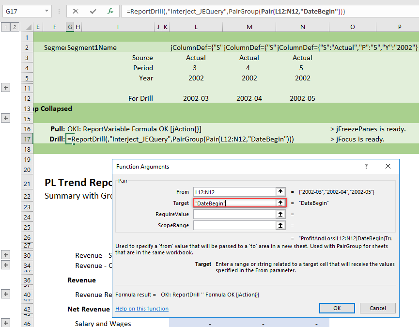
Step 5: Now, type DateBegin in the Target argument to establish the target cell that will receive the month. DateBegin is a Named Range in the target sheet. Named Ranges are used in MS Excel to assign a name to a specific cell, such as G15. You use Named Ranges in your drill in case rows or columns are changed in the target worksheet where the address of the target cell changes. By using Named Ranges, the drill will continue to find the correct cell to place the month into.

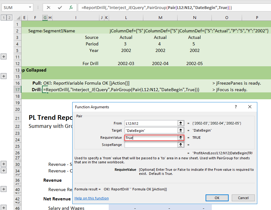
Step 6: Now, type True in the RequireValue argument because the From value must exist to trigger the drill. There would be no point in drilling to the target report without filtering for a specific month. The True value is not required since, if left blank, True is assumed. Since this drill exercise will have other Pairs() that are not required, it is good practice to specify it explicitly in this case.

Note the next argument, ScopeRange, is not used. It is an outdated argument.

Step 7: Now that you understand how to define a Pair, you have many more to create. The target report has several filters that make use easier when employed separately and in drilling to the report. You need to add a few more values to pass to the new report and clear the remaining filters that are not used in this drill. This is a key concept for Interject drills. A report can be used by itself for its own purpose, but it can also be used as a drill from other reports.

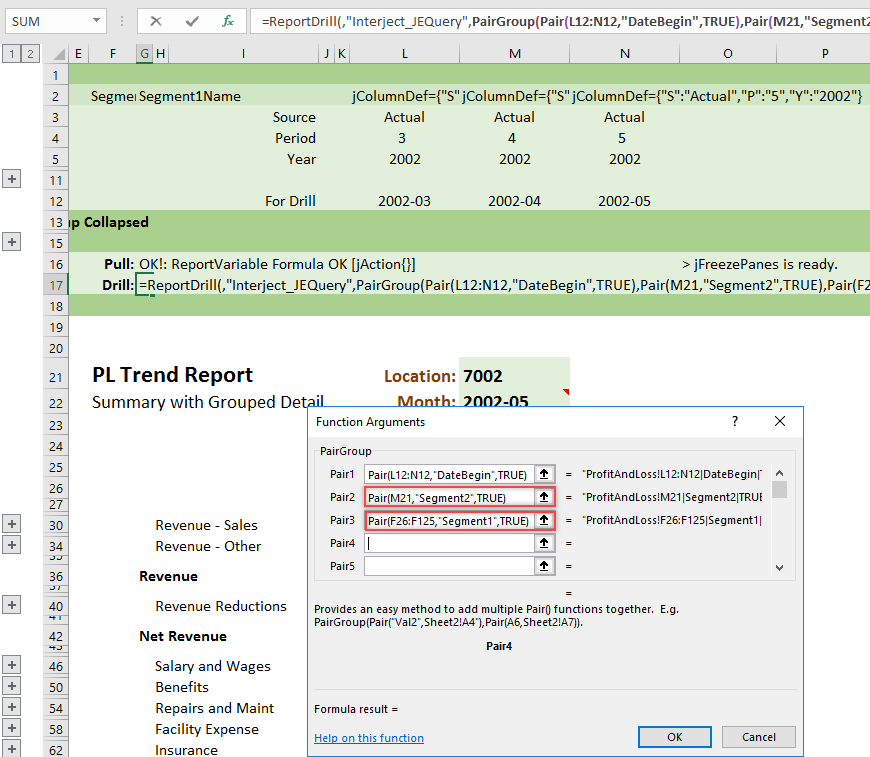
Now let's use the Function Wizard to edit the PairGroup() function by clicking on it in the Formula Bar as seen below. This will make it easier to create more Pairs() that will clear out the other filters in the target report.

Step 8: You have two more values to pass, the Location and the Account. Type Pair(M21,"Segment2",TRUE) into Pair2, which will pass the Location into the next report, and type Pair(F26:F125,"Segment1",TRUE) into Pair3, which will pass the Account or Account Group into the next report.

Note: Excel is picky about Quotation marks so please ensure all your formulas have Straight Quotation marks (instead of Smart Quotation marks) in order for the formulas to work.

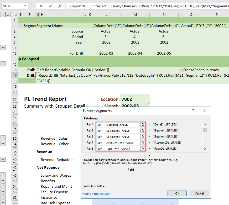
Step 9: You need to make sure the other filters in the target report do not interfere with the drill, so you will set this next group of Pair() functions to bring over blank values. In the Pair() functions you are going to set the From arguments to blank (""), and you will make the RequireValue argument FALSE . Both steps 9 and 10 are adding Pair functions that clear out the unused filters. This is best practice, but steps 9 and 10 can be skipped since it will not impact the limited scope of this exercise.

Enter the following pairs as shown below:

Pair("","DateEnd",FALSE) into Pair4

Pair("","Segment3",FALSE) into Pair5

Pair("","Segment4",FALSE) into Pair6

Pair("","AccountDesc",FALSE) Into Pair7

Pair("","TypeDesc",FALSE) Into Pair8

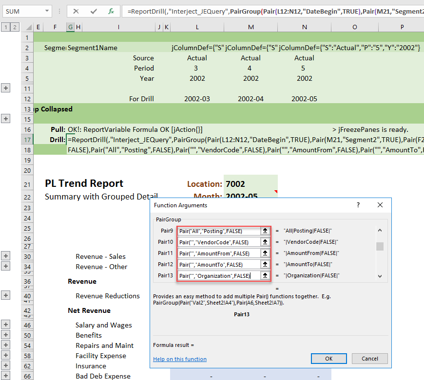
Step 10: There are still more filters to blank out for the target report. Continuing typing the following.

Pair("All","Posting",FALSE) into Pair9

Pair("","VendorCode",FALSE) into Pair10

Pair("","AmountFrom",FALSE) into Pair11

Pair("","AmountTo",FALSE) into Pair12

Pair("","Organization",FALSE) into Pair13

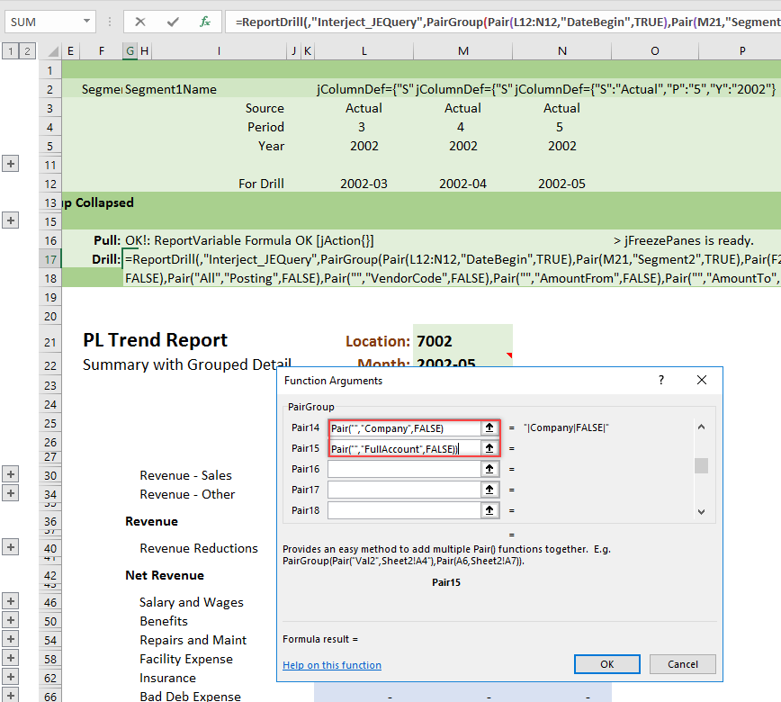
There are two more pairs to enter. Scroll down and type:

Pair("","Company",FALSE) into Pair 14

Pair("","FullAccount",FALSE) into Pair 15.

After these, you are through adding the Pair() functions.

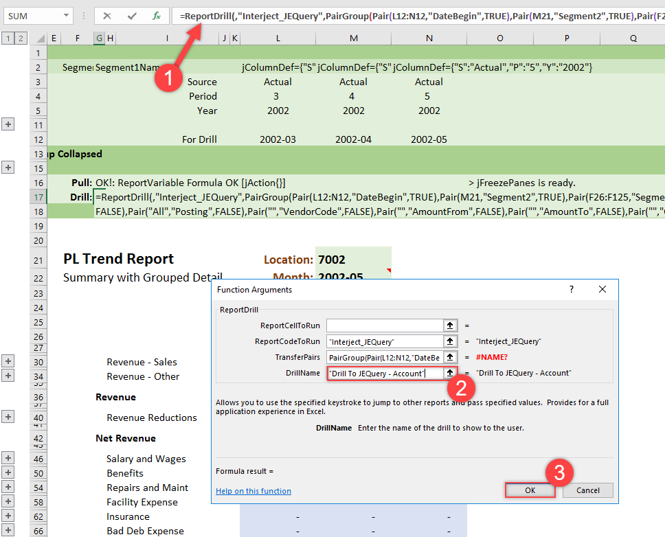
Step 11: You need to name the drill so it is clear for the users. Click on G17 and select the fx to bring up the Function Wizard. Input Drill To JEQuery - Account into the DrillName and select OK to finish creating the drill.

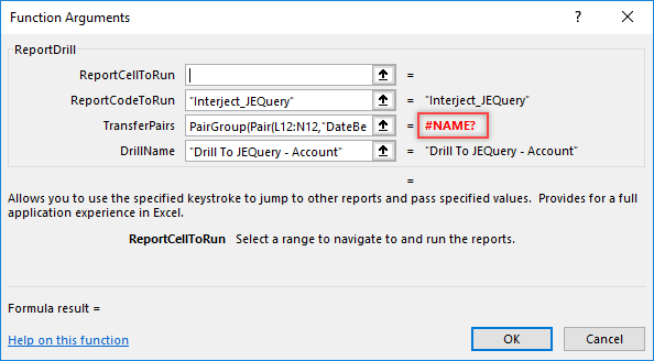
When you click away from TransferPairs, it shows a red #NAME? to the right of the input area. That looks like an error, but it is simply a small bug in Microsoft Excel, which will hopefully be addressed.

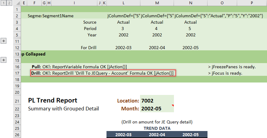
Step 12: You successfully created a Drill to the Journal Entry Query report from the financial report.

Executing the Drill

Step 1: Use Pull Data to pull the report. You can leave the panes open for the moment. They will not affect the drill feature.

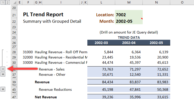
Step 2: Scroll down to the Revenue - Sales row on line 32 and click the plus sign so it expands to show the accounts. There should be several accounts listed as shown below.

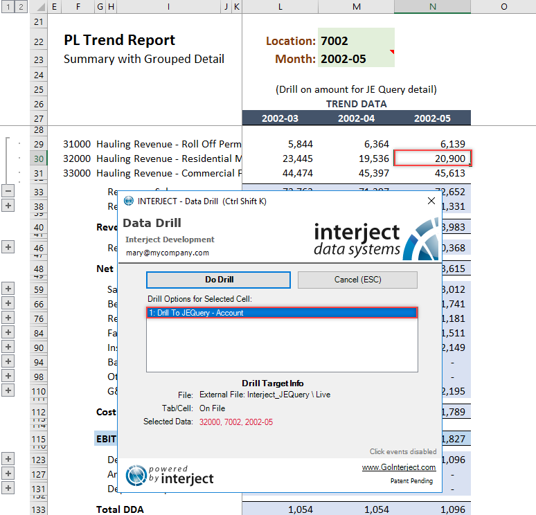
Step 3: Click the amount $20,900 which is for account 32000 in May 2005. You can then use the keystroke Ctrl + Shift + K or use the Drill on Data menu item to bring up the drill options.

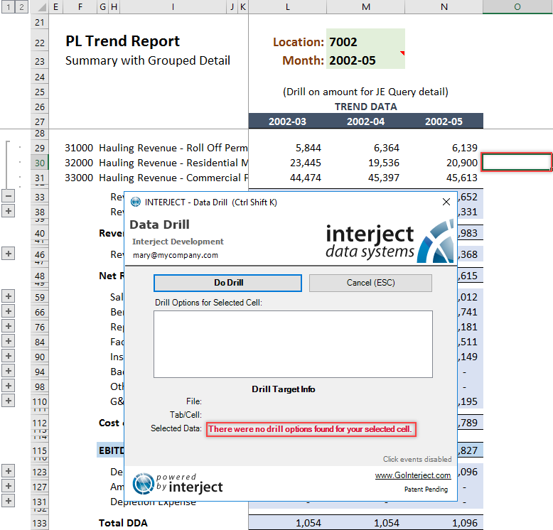
Notice that if you close the drill window and try to drill on column O, there will not be any drill options. The work you did above helped set the scope so the drill only works on the appropriate cells.

Step 3: The animated GIF below shows the drill completed. The panes are frozen again. The drill selects the amount for account 33000 for March 2002, then does the drill on amount $44,474. The JE Query report provides the detail to support the same amount.