Modify: Financial Report

Overview

Financial reports can sometimes share the same row or column configurations. Rather than creating a new report, it is often easier to modify an existing one. For example, you might be using a monthly trend report which could easily be modified to accommodate a budget-to-actual comparison report, showing monthly and year-to-date differences. This Walkthrough will illustrate how to make these changes.

If you are following the Training Labs, this report file can be found in the Report Library at Training Labs > Lab 2 Modifying Reports > Lab 2.3 Financial Report.

Using Column Definitions

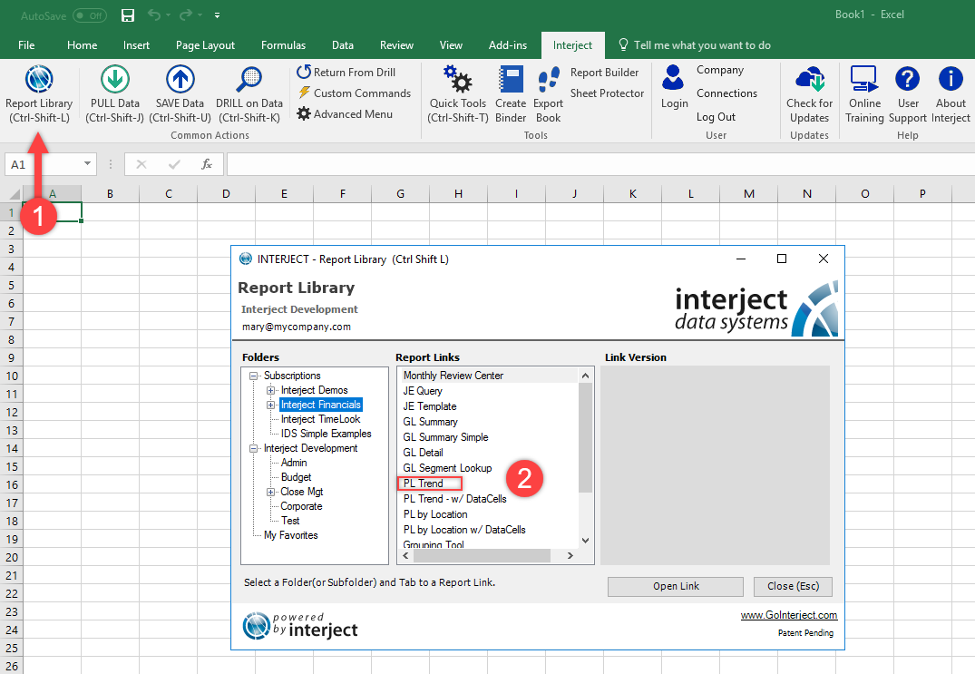
Step 1: Open the PL Trend report from the Interject Financials folder of the Report Library.

Step 2: Once the report is open, select the Freeze Panes menu in the View tab, and choose Unfreeze Panes.

Enter 7002 in the Location filter in cell M22 and month 2002-05 in cell M23. In the current report, values in L4 through N5 will populate based on the month entered. These cells were configured with spreadsheet formulas to automatically change based on the month entered.

The jColumnDef() formulas in cells L2 to N2 are important to understand. They exist in the Column Definition row 2, so Interject understands what financial values to present for that column.

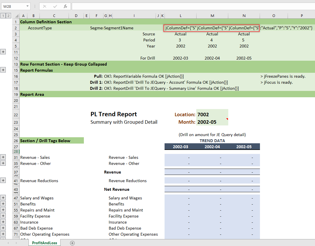
Notice that jColumnDef() draws its parameters from the cells that it has been designated to take values from. In this case those cells are right underneath the formula. Here, jColumnDef() is only referencing a Source (Actual or Budget), a month period, and a year. However, it is designed to handle currency and other reporting dimensions as well.

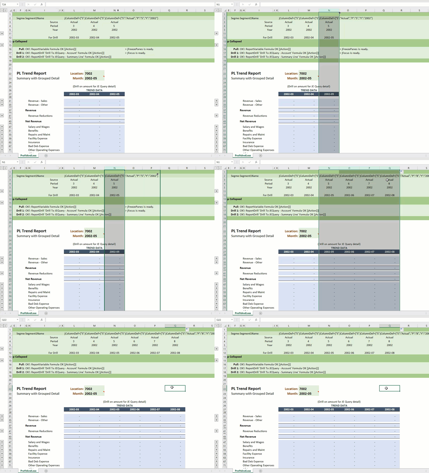
Step 3: Expand the trend 3 more months as illustrated in the following animated GIF. Select column N and drag its anchor 3 columns to the right. Note that the Column definitions carry through the new columns you made just by dragging the previous one. This way, you add more columns to to the report without manually typing formulas.

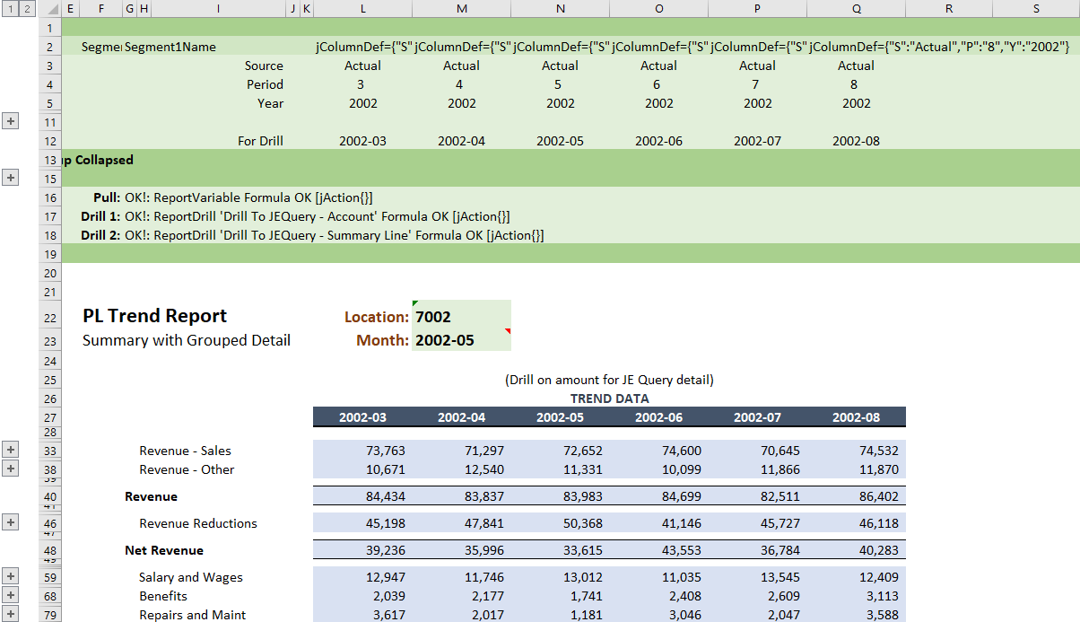
Step 4: With the new columns added, use the Pull Data menu item.

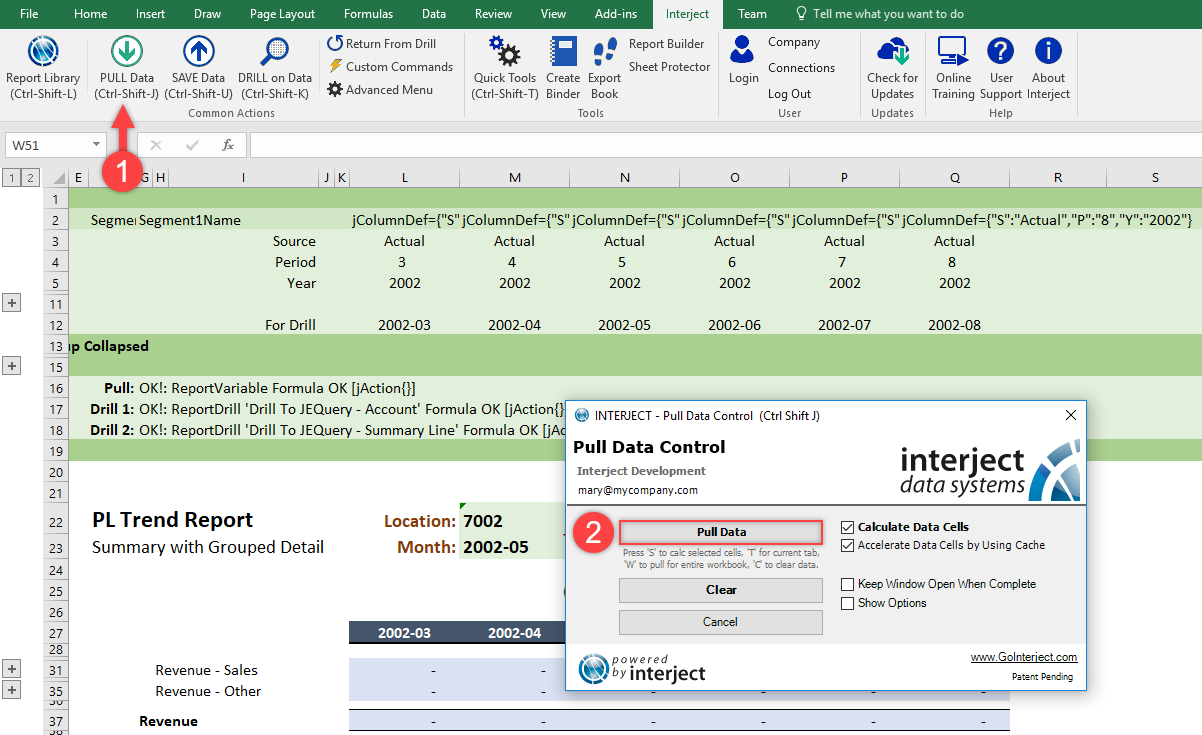
You can see that even with the expanded sheet, the data populates in the desired areas just as it should.

Preparation Cleanup

Now that you understand Column definitions a bit better, modify the report to create a budget to actual comparison report. Before doing this, cleanup the report to prepare it for the modifications you will make.

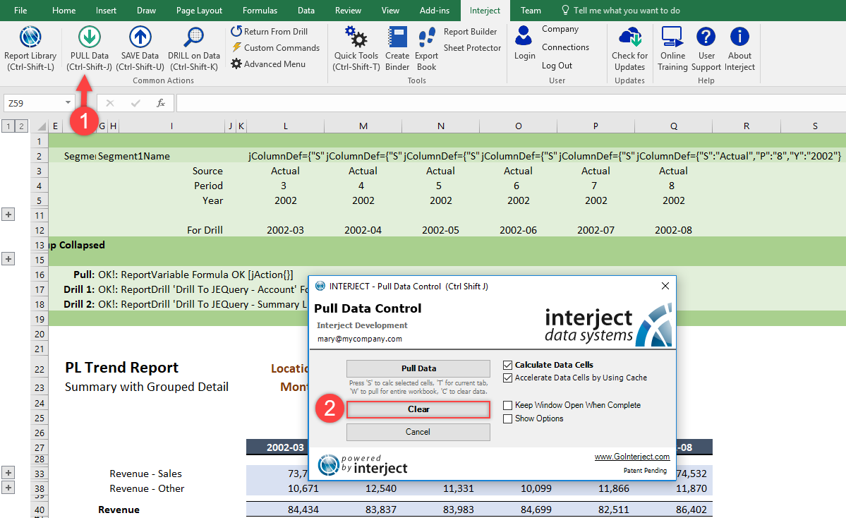
Step 1: Now, use the Clear button to remove the data on the report.

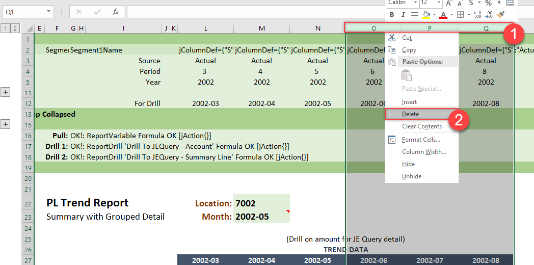
Step 2: Next, you will select the columns you do not need and right click to delete them. In this case delete Columns O through Q.

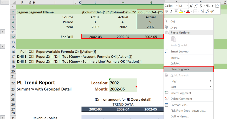
Step 3: Clean up the Column Definition area so the changes are easier to make. First, delete the For Drill row to simplify the changes as illustrated below. Delete the column definition area for the third column since column N will contain a formula for difference and thus will not need a column definition. Do this by selecting and deleting cells I12, L12, M12, and N2, N3, N4 and N5.

Setting up Budget to Actual Comparison Report

Now that you have cleared those cells, begin by modifying the report to create a Monthly Comparison Report.

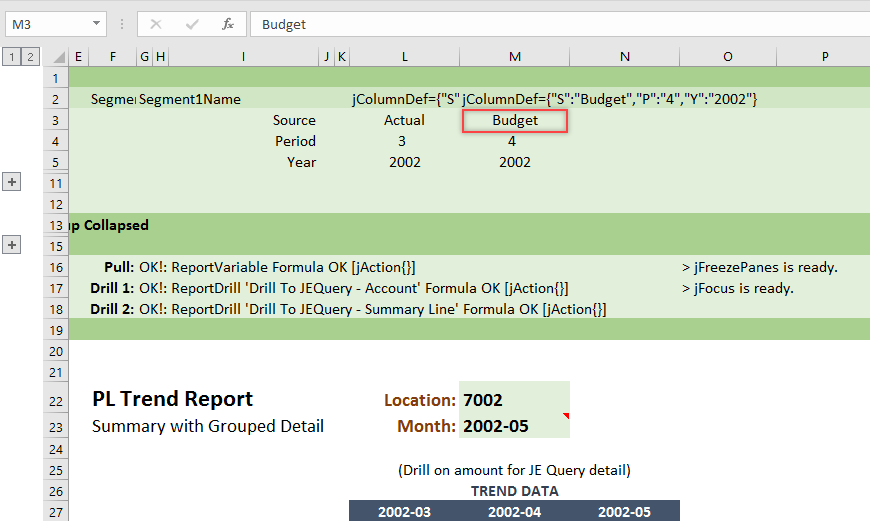
Step 1: To begin, change the Source of column M to Budget so it can be compared to Actuals. Enter Budget in M3.

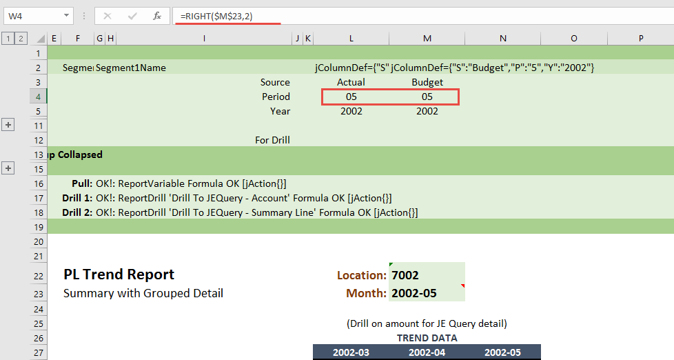
Step 2: Next, you will need to define the Period. Type =RIGHT($M$23, 2) into the function field for cells L4 and M4. This way, if a user changes the month in the report, it will change in the Column Definition as well. Add the $ symbol in the formula so that it will lock in place if the formula is copied later.

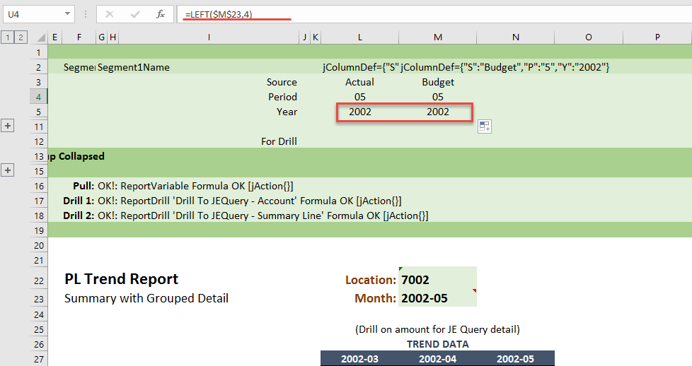
Step 3: Now, define the Year. Type =LEFT($M$23, 4) as the function for L5 and M5, so if a user changes the year in the report, it will change in that Column Definition as well.

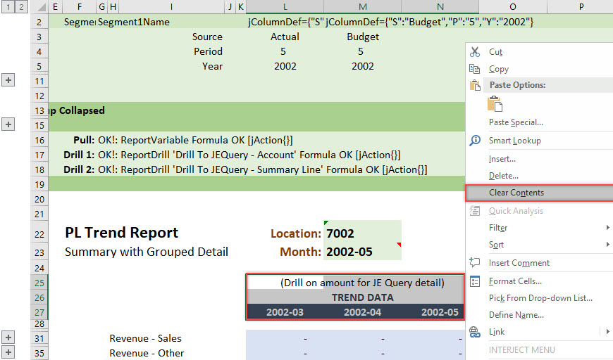
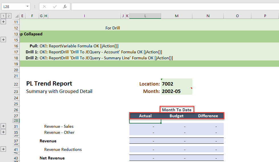
Step 4: Now, rename the column labels in rows 25 to 27 so they will more accurately describe what they represent. First clear the range L25:N27.

After the old content is deleted, add the new descriptions for the column labels. Type Actual in cell L27, Budget in M27 and Difference in N27. Type Month to Date in M26.

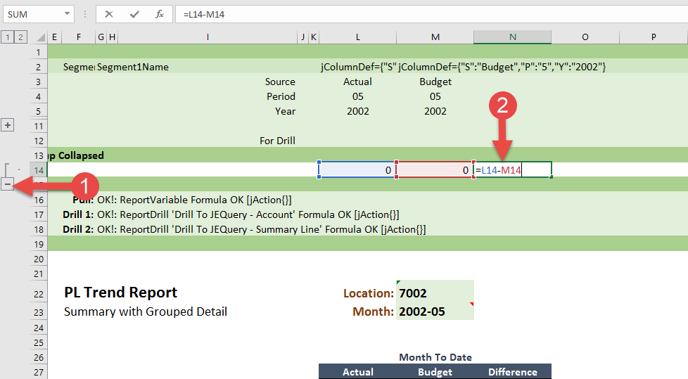
Step 5: Now, set up the difference formula for column N. First, expand the grouped row in the Formatting Range section in row 14. Type =L14-M14 into cell N14. This will populate the difference Column with the difference between column L and M.

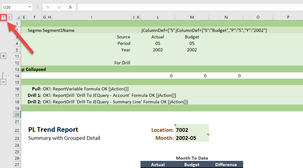
After that, select the 1 icon to close all the groups. See the red arrow in the screenshot below. This report was specifically built to be pulled with the groups closed, so it should be collapsed before the report is pulled again.

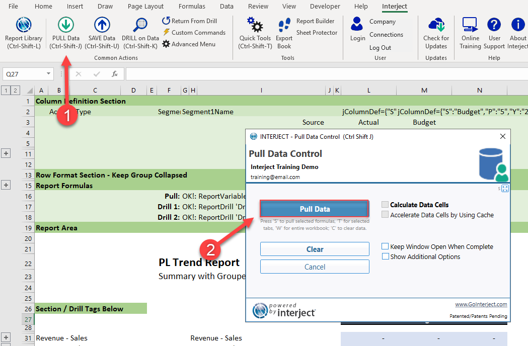
Step 6: Now that you have all of the columns set up for the Budget to Actual Comparison Report, you can pull the data. Just click Pull Data in the ribbon menu.

The new month-to-date difference report columns should populate as expected. Refreeze the pane on cell L28 and the report will look like the image below.

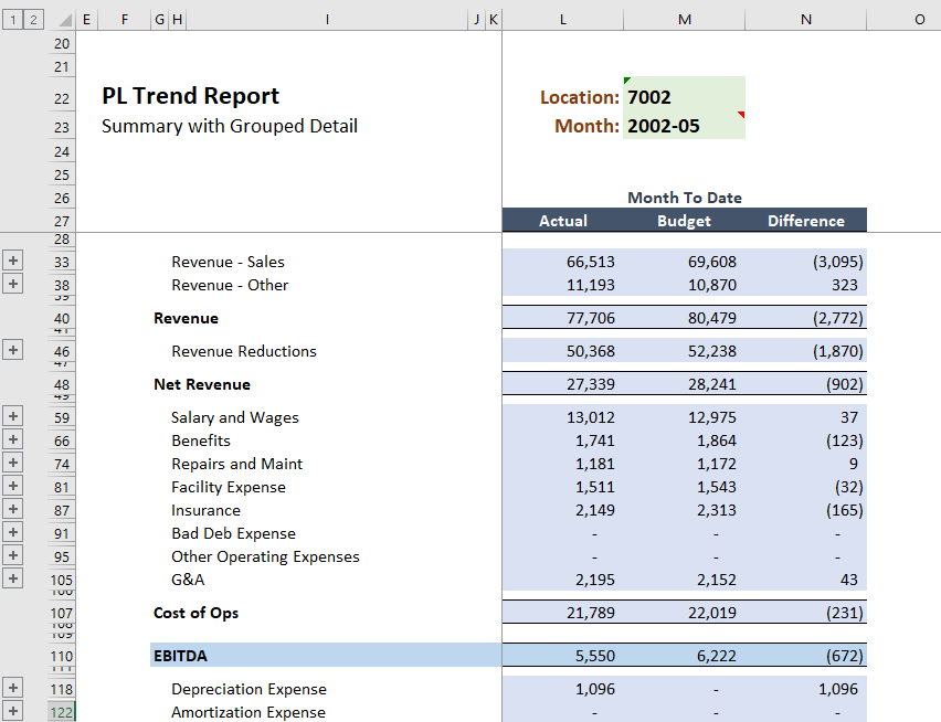
Creating a Year to Date Budget to Actual Comparison Report

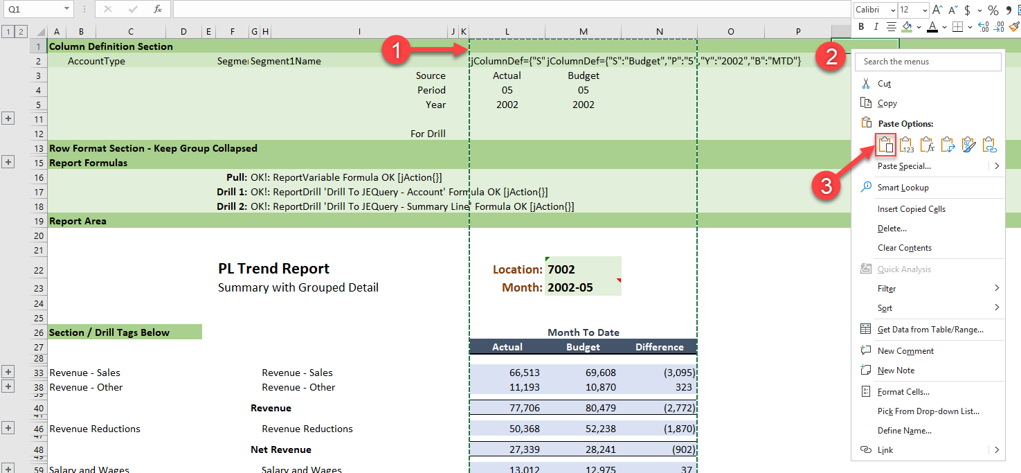
Step 1: Now change your Budget to Actual Comparison Report to show the monthly difference as well as the year to date difference. You can do this by first selecting columns L through N, then copying and pasting them in Column Q. This will give you a broader view of the data. Once completed, you can view not only the month you are asking for but also the year.

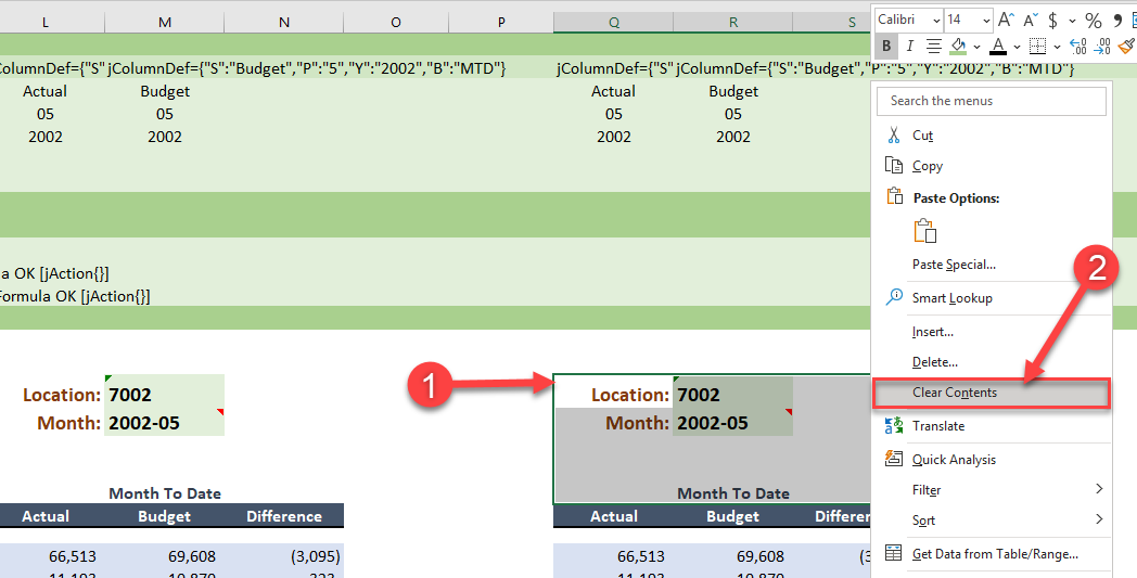
Step 2: Now delete the unnecessary data. Select cells Q21:S26. Right-Click on the area and select Clear Contents.

Now copy a blank cell and past it over what you do not need. Change the name of the table to a more accurate name, like Year To Date.

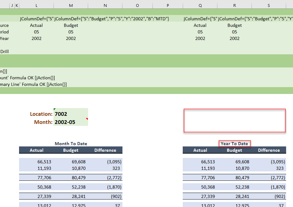
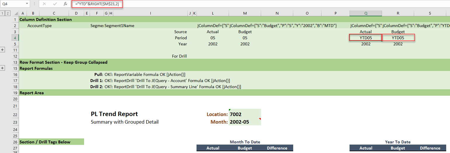
Step 3: Now, change the Period for the Year To Date so it will show the actual Year to Date. You can do this by typing ="YTD" & RIGHT($M$23, 2) into the function dialogue for cells Q4 and R4.

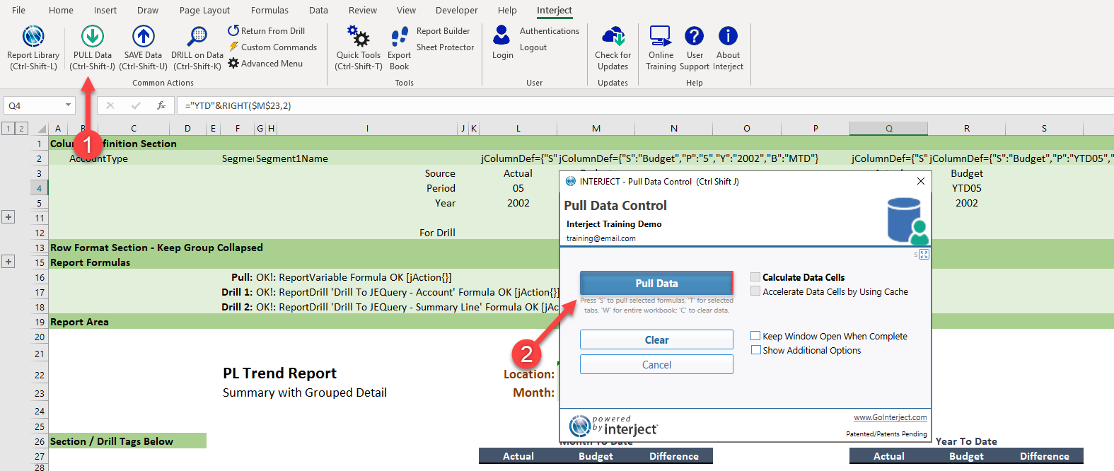
Step 4: With this done, re-pull the data.

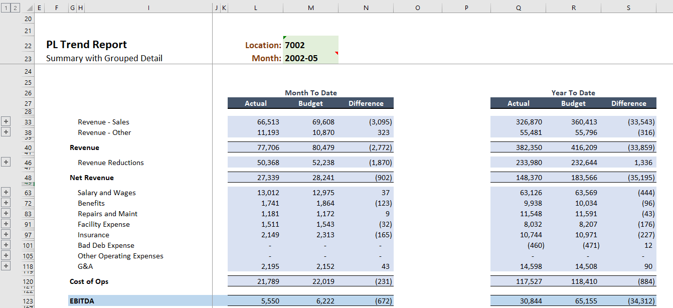
After the pull, refreeze your panes. The new Year to Date Budget to Actual Comparison Report will look like this.

Finally, clear the report and save the file to the Report Library "My Favorites" folder. (For detailed instructions on how to save a file to the Report Library, see here.)