Create: Financial Variable Report

Overview

The ReportVariable() function is ideal for financial reports since it directs data into multiple specified ranges of a report that can grow and shrink with the data. In this example you are going to use the Financial Cube (FinCube) Data Portal to create a financial statement from scratch. First you will use the ReportRange()formula to review the financial group summaries for a location. With the financial groups retrieved, you will than expand to create a subtotaled financial statement so each subtotaled detail will expand and shrink with the data.

If you are following the Training Labs, this is Lab 3.5. Note: The Report Library at Training Labs for this lab will be blank as you are creating a report from a new blank Excel sheet.

Pulling Financial Data With FinCube Data Portal

To get started you will need to learn how to pull financial data from the Interject Financials for Spreadsheets application. You will initially use ReportRange() to pull a simple list of balances by account.

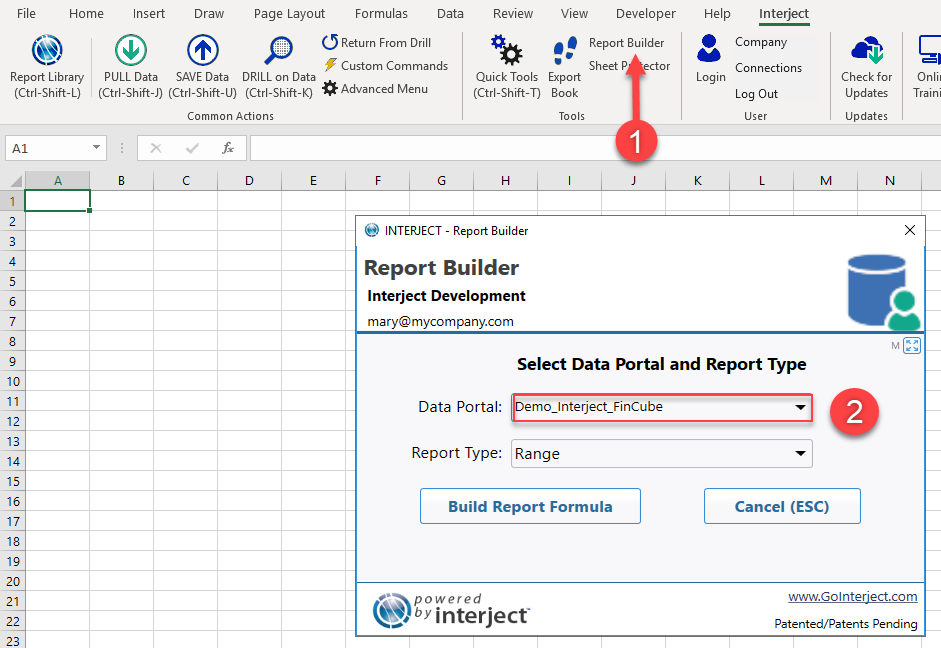
Step 1: Open a new worksheet and choose the Report Builder from the Interject ribbon. For this example you will be using the Interject_FinCube Data Portal. Select Demo_Interject_FinCube from the Data Portal list and click the Build Report Formula button.

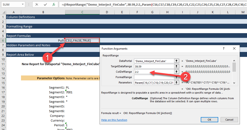
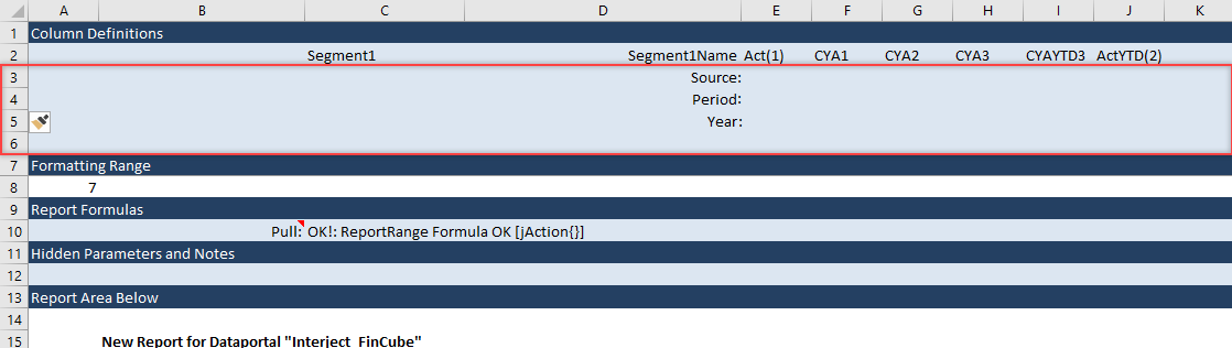
Step 2: The worksheet should look similar to below. A ReportRange() formula should be setup in C6 and its related parameters were placed starting in row 16.

This Data Portal is special and will not show all the available columns by default if you do not have a Column Definition defined. There are simply too many combination of column options to present. So you need to setup the Column Definition range first.

Select cell C6 and click the Fx button. Set the ColDefRange argument to 2:2 as shown below. This row is where you will specify the columns for the report.

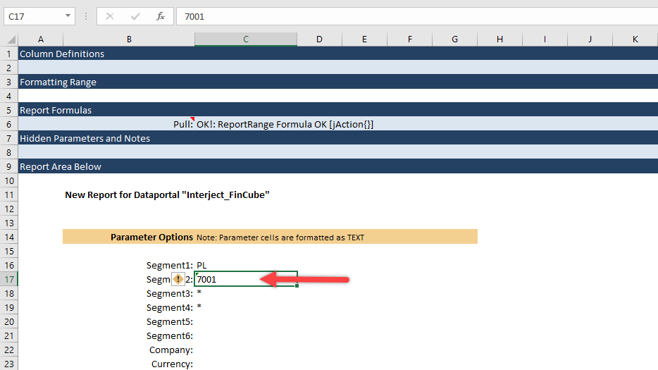
Step 3: Adjust the default filters and the Column Definitions to match the intended report. In cell C17, change the Segment2 filter from 7001 to 7002. Segment2, in this demonstration demo, represents a location or a cost center.

Before:

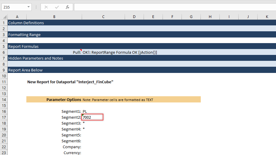
After:

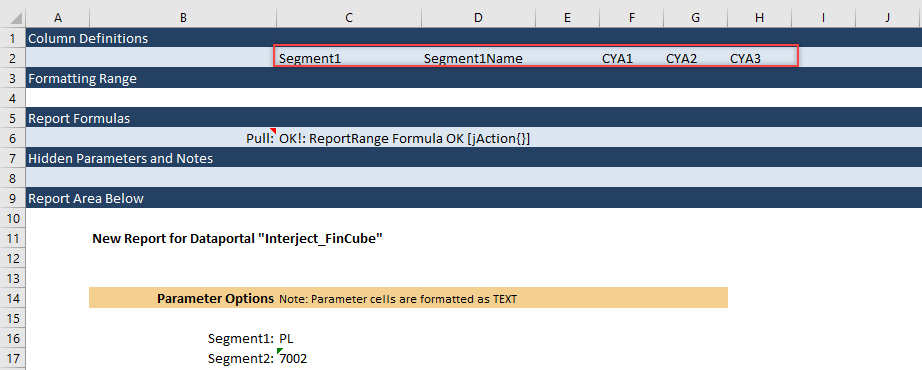
Continue to input the Column Definitions. Enter Segment1 in C2, Segment1Name in D2, CYA1 in F2, CYA2 in G2, and CYA3 in H2. Segment1 in this demonstration represents a general ledger account. The notation CYA1 represents an amount, specifically for the C_urrent _Y_ear _A_ctuals for month _1, January. The notation options for amounts are further discussed in this link FinCube - The Financial Cube but you can go through several examples in this exercise.

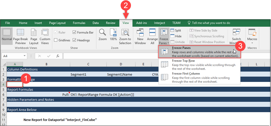
You need to do one more thing before pulling the data. Since this worksheet is very tall, freeze the panes in row 3 so you can keep the column headers in view as you are looking at the data that results.

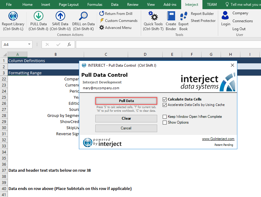
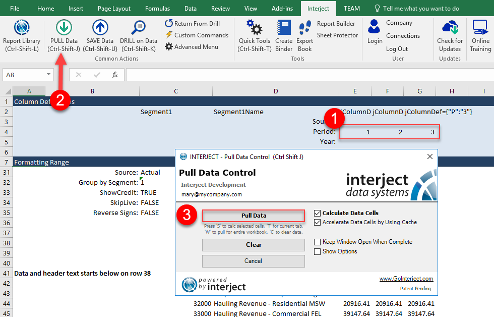
Step 4: Pull the data to see the results.

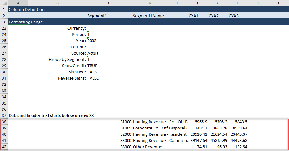
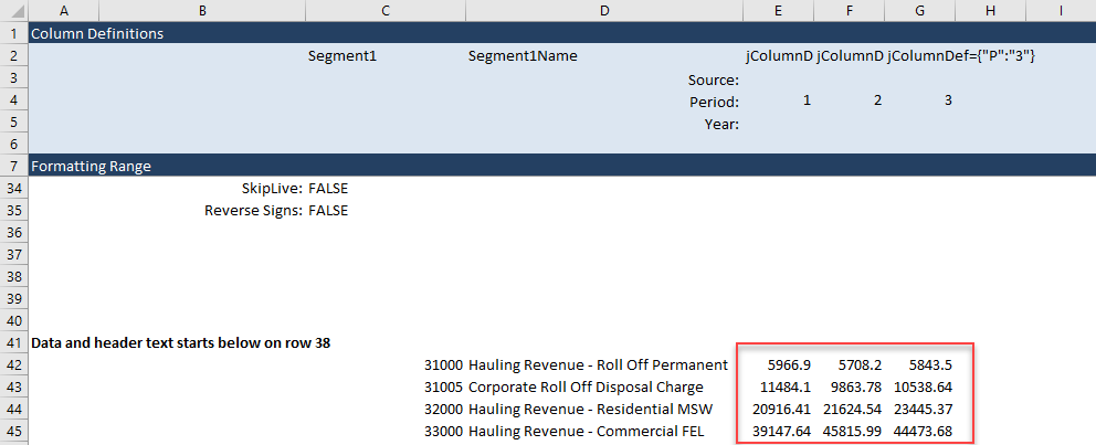
Down in row 38, scroll to the data that was inserted. There are account descriptions and amounts for Jan 2002, Feb 2002 and Mar 2002.

Change the width of column D to 35 so you can see the full account descriptions.

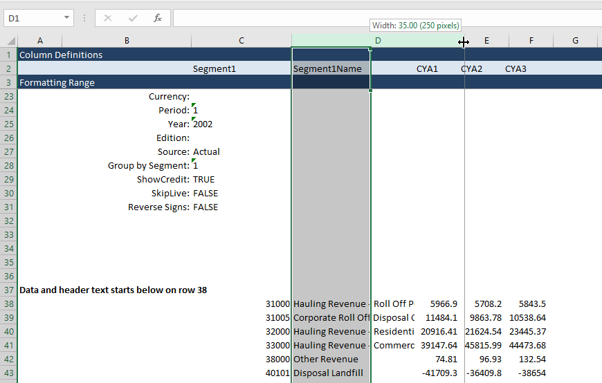
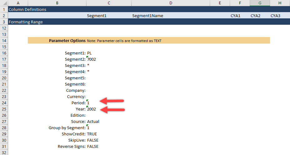
You can answer the question on how you are viewing the amounts were for the year 2002. In cell C25, it shows the filter that was used and it is set to 2002. This will define what CYA (current year) is. There is also LYA (Last Year Actual) and others noted in the documentation link FinCube - The Financial Cube. Notice that you also defined a period 1 in cell C24. This will be the default period that you will use in the next notation example.

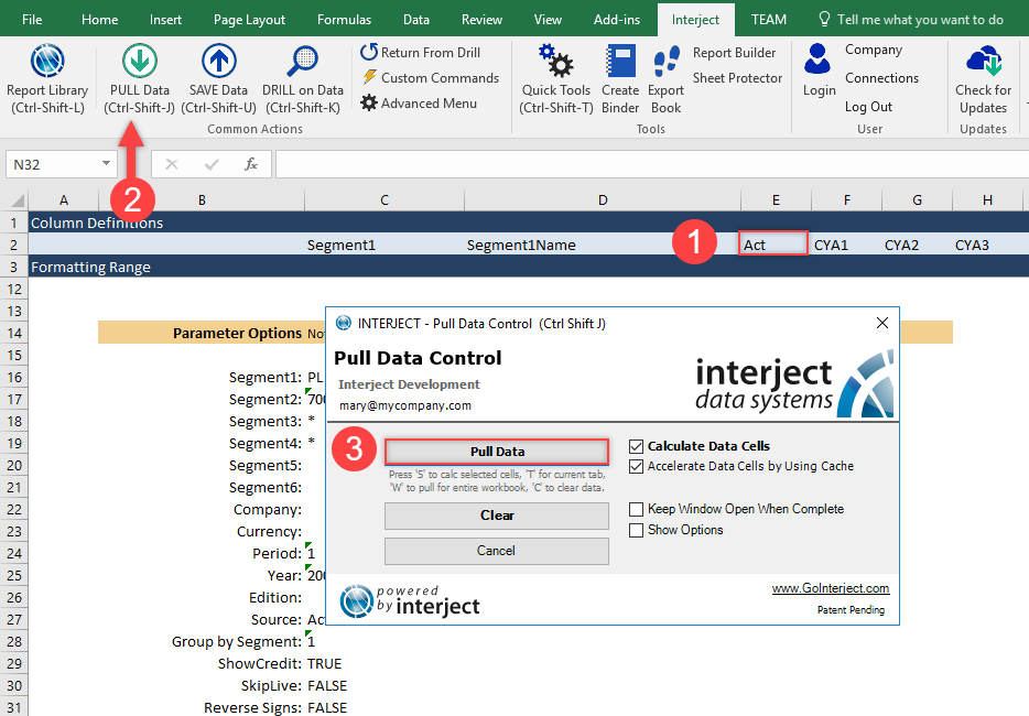
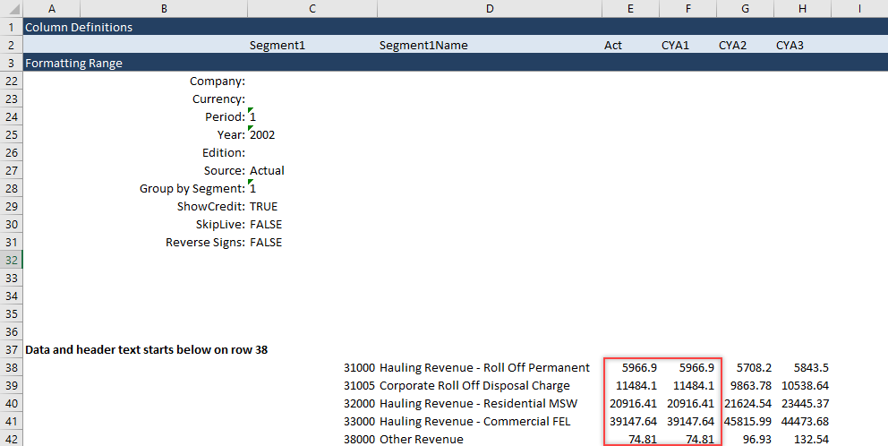
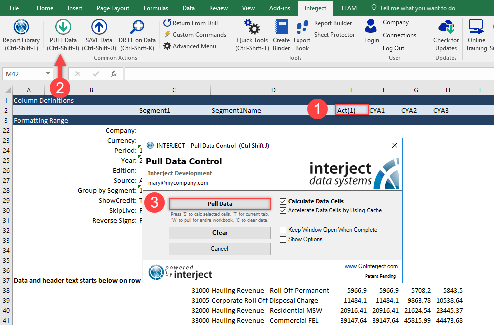
Step 5: In cell E2, type in Act, short for Actuals. Then re-pull the report.

In column E (from the Act notation), you can see is the same as column F (from the CYA1 notation). They are both for Jan 2002. The Act represents actual for the current period that was specified in the period filter noted above.

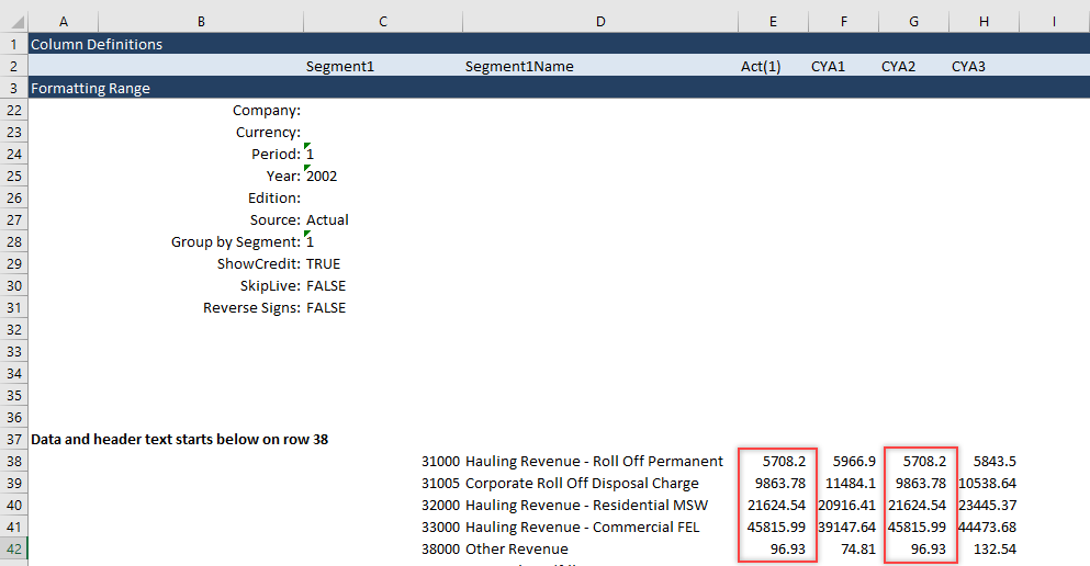
Go further and change cell E2 to Act(1). The suffix (1) will adjust the period by one. By adding this the amounts returned should equal column G, Feb 2002. (You can use (-1) to go the other direction for previous months. You can review further notation options in the link FinCube - The Financial Cube.) Re-pull the data.

Both columns E and G are the same amounts, as expected.

Step 6: In cell I2, type CYAYTD3. CYAYTD stands for Current Year Actual Year To Date. The (3) signifies the amount for the 3rd month (March). In cell J2 type ActYTD(2). This stands for the Actual Year To Date and the (2) means add 2 months to the current month. So 2 months past January is March. Re-pull the data again.

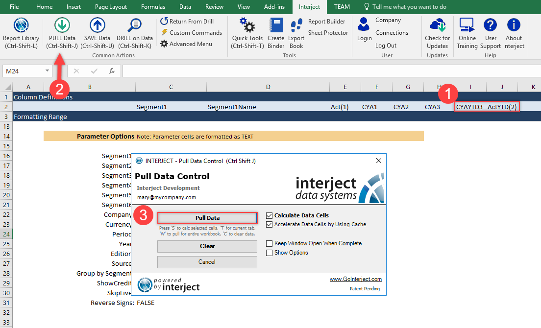
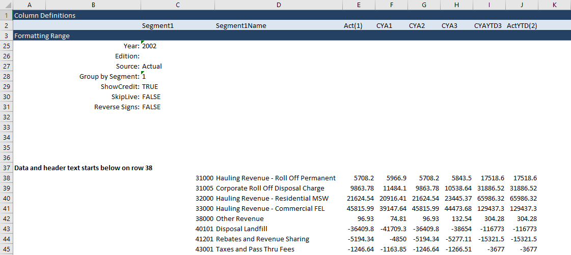
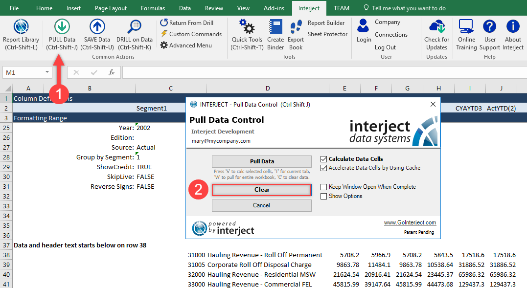
As seen in the below screenshot, both CYAYTD3 and ActYTD(2) values match.

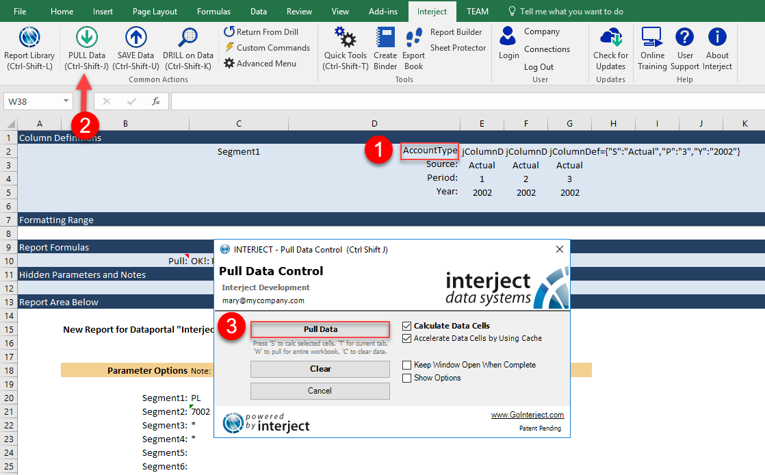
Before moving to the next step, clear out the data. Click the Pull Data menu item and choose the Clear button and the data should be removed as shown below.

Step 7: Move on to the next amount notation that is much more flexible. By using a helper function jColumnDef() in Column Definitions you can define the columns illustrated above and go much further in defining what each column should be. First make room to use this helper function. Insert 4 rows under row 2. Now label the new rows. In cell D3, type Source:. In cell D4 type Period:. In cell D5, type Year:. Format D2:D5 to be right aligned as well since that will look better.

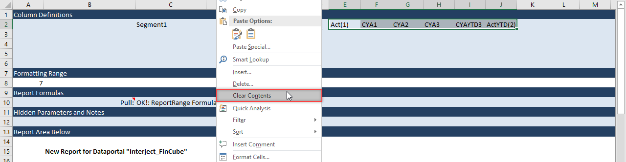
Next remove the previous amount notations in cells E2 through J2. Select E2:J2 and clear contents as illustrated below.

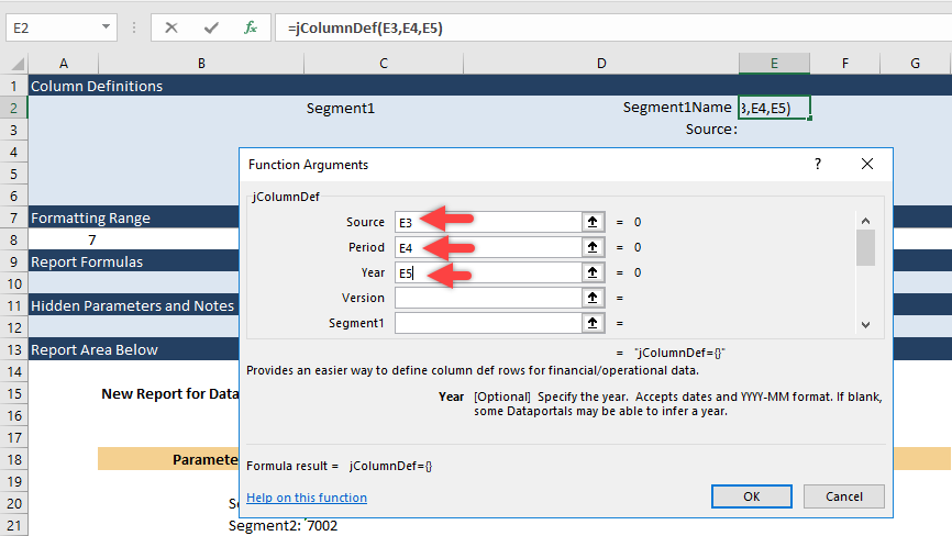
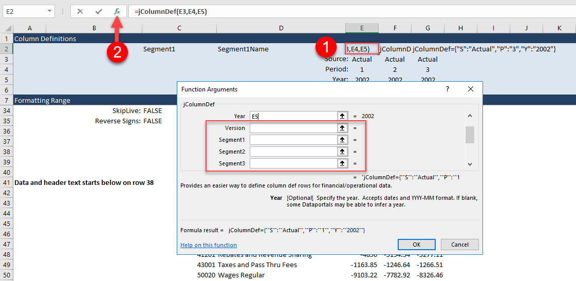
Step 8: Now insert the helper function, jColumnDef() into E2. Type =jColumnDef() in E2 and click the Fx button to bring up the Function Wizard. The arguments for the jColumnDef() function closely match many of the parameter filters of the Data Portal starting in row 20 of the spreadsheet.

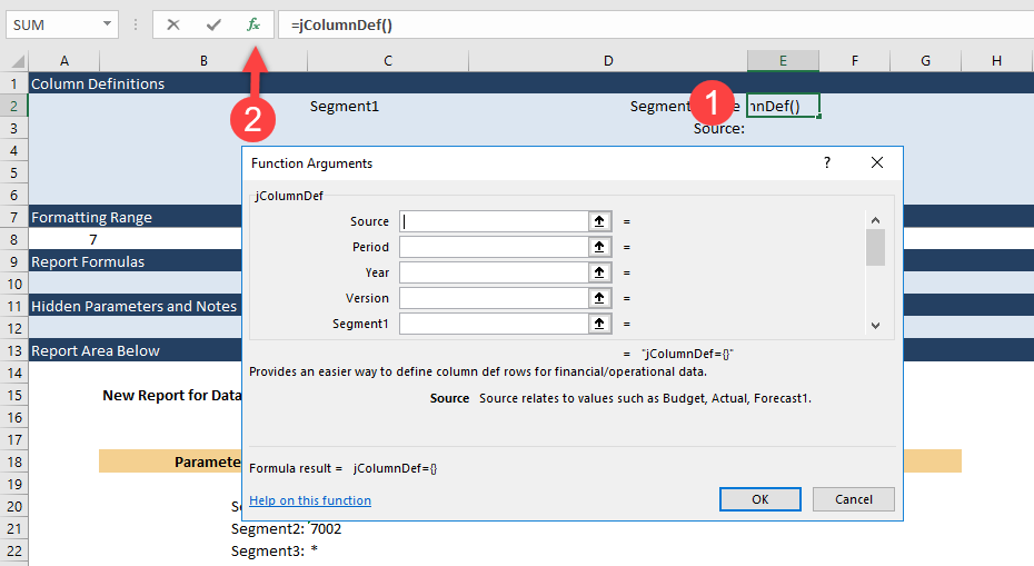
Go ahead and type E3 for the Source argument, type E4 for the Period argument, and type E5 for the Year argument.

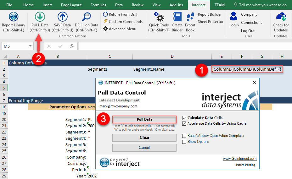
Copy the existing jColumnDef() formula to F2 and G2 so you have more columns to work with. Then pull data using the Pull Data menu item.

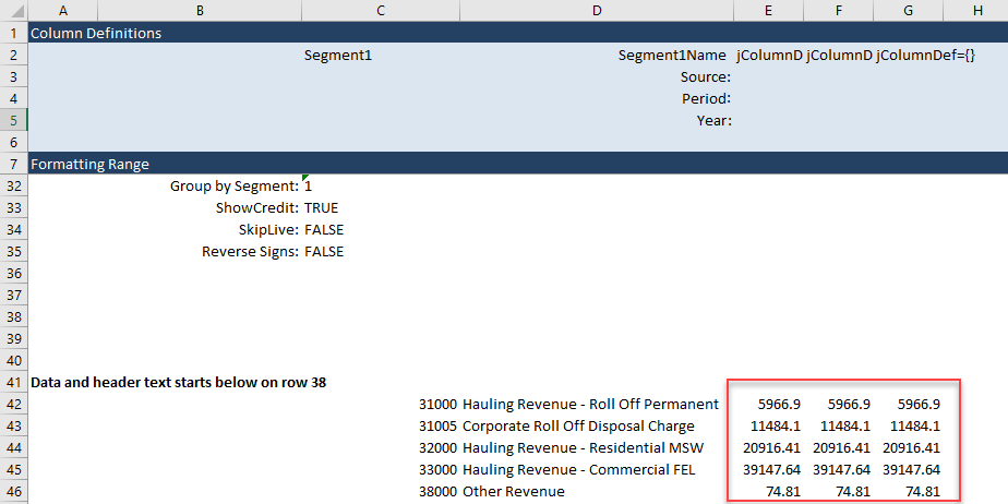
Columns E, F and G are all the same amounts. They are amounts related to the Data Portal parameter filters starting in row 20 of the spreadsheet. Since the JColumnDef() function added no additional values for its arguments, it let the Data Portal parameters defaults remain.

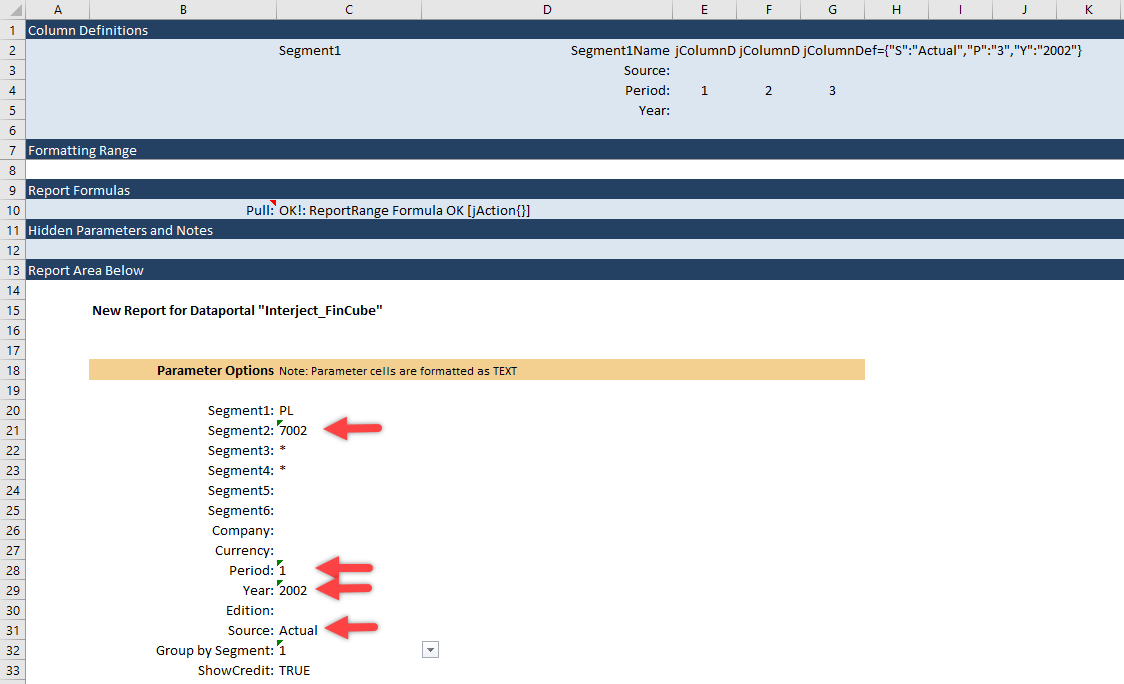
Those filters have defined the totals to be: PL accounts only (which is defined as all the Profit and Loss general ledger accounts); Segment2 (Location) = 7002, Period=1, Year=2002, and Source = Actual. If you do not setup any arguments for the jColumnDef functions, it does not refine it any further.

It is important to understand how both sets of filters interact. The jColumnDef() arguments serve as filters for the column while the Data Portal parameter filters in the spreadsheet are default filters when not defined by JColumnDef().

Step 9: To expand on the jColumnDef() filter arguments, type in specific values for jColumnDef() to reference. In cells E4, type 1. In F4, type 2. in G4, type 3. Then re-pull the data.

The resulting data is the same data you pulled for CYA1, CYA2, and CYA3 above. The Period argument for jColumnDef() overrode the Data Portal filters and changed how the column was presented.

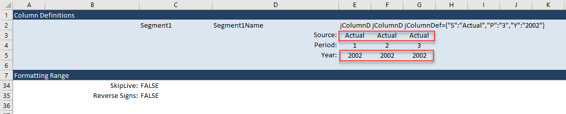
For clarity, type in all the jColumnDef arguments like shown below. Type Actual in cells E3, F3, and G3. Then type 2002 in E5, F5, and G5. This will not change the data that is pulled since it was already setup that way in Data Portal parameters, but it is easier for a report writer to see what is being presented.

Before moving on, bring up the jColumnDef() Function Wizard again. Click on cell E2 and click the Fx button to view the arguments below Year. These are other dimensions/segments that can be used to define what each column holds and you can use advanced filter notation to handle complex arrangements. Columns could hold different cost centers, geographic regions, currencies, etc. See FinCube - The Financial Cube for further details on the filter syntax that can be used.

You should have a much clearer idea on how to use notations to bring in the balances that you need for reports. You can continue to shape the existing report into a Profit and Loss report.

Preparing the Row Format

To setup the financial report you need to first get the financial groups that will be used as subtotal sections. Then you need to create the final row format with the subtotaled sections that you need for the report. In most cases you can use an existing report that has the correct row format and change the columns. In this example you will start from scratch. It will be more work up front, but it can be re-used for future reports.

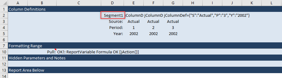
Step 1: First, you need to update the report to show the Account Type, which is the financial grouping you will use in cell D2, change Segment1Name to AccountType and re-pull the data.

As seen in column D, you get the AccountType text and the account group in column C. These are the groups you need, but you want a unique list. Clear the data again.

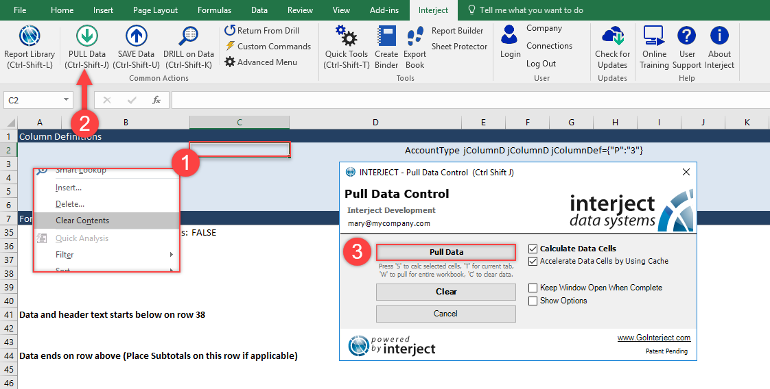
Step 2: Once the clear is done, remove the value in cell C2. By removing the Segment1 from the Column Definitions, the amounts will be summarized only by the Account Type. Re-pull the data once again.

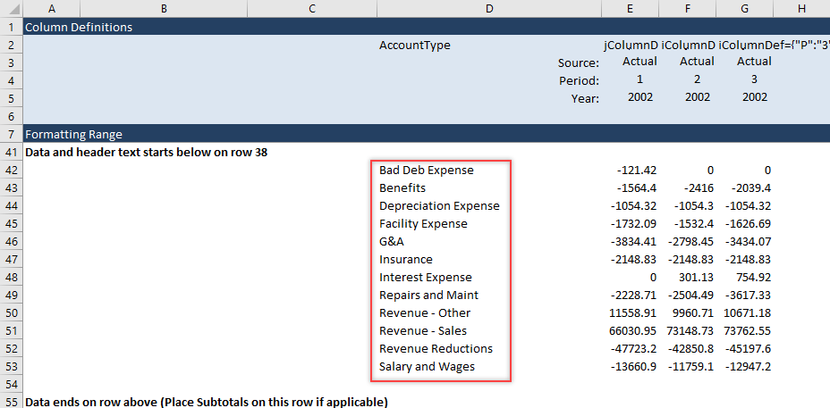
The report will look like below, showing the full data results of the amounts by account type.

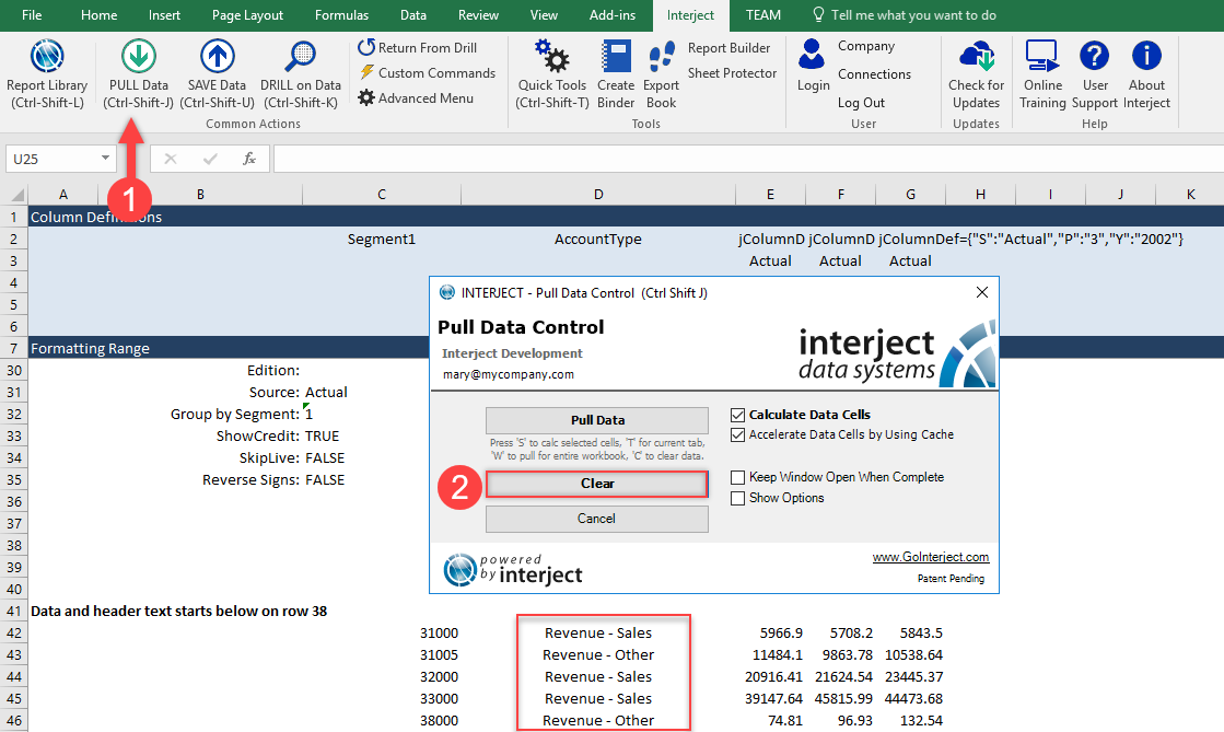
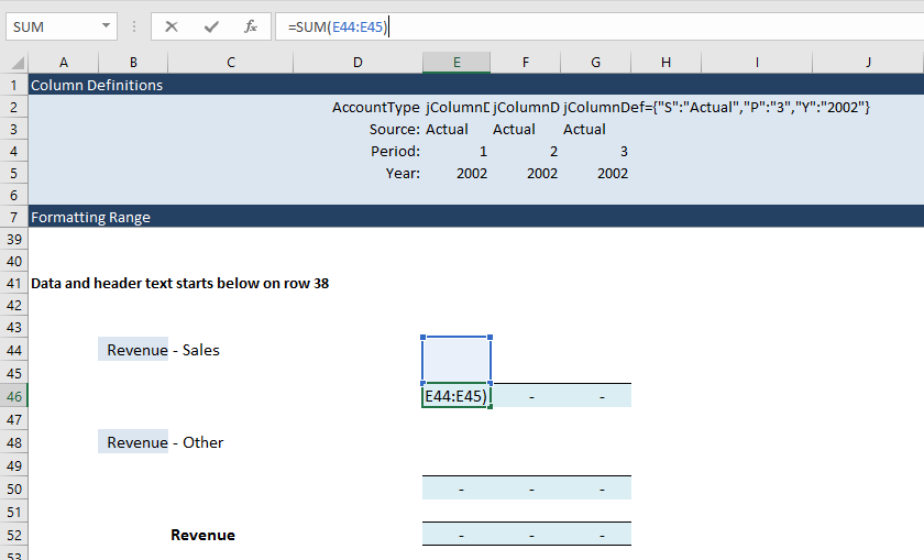
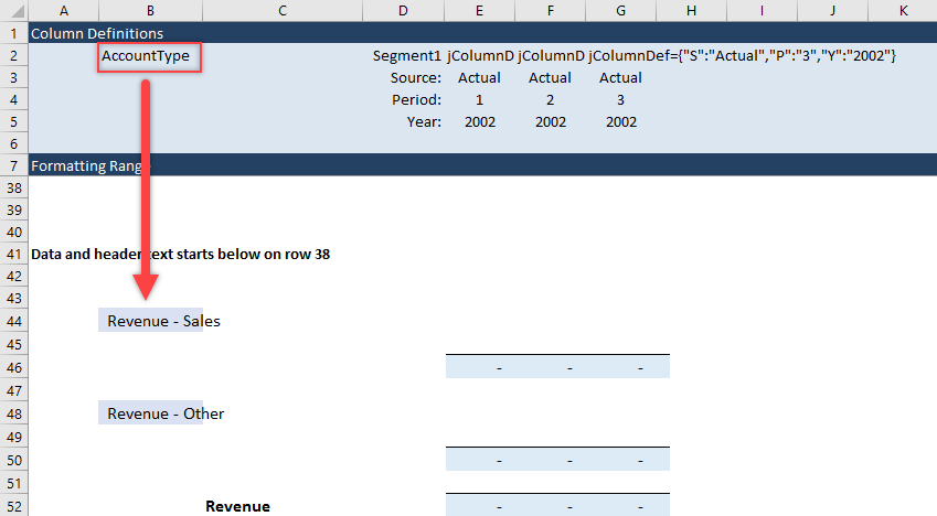
Step 3: Now you have the Account Types, you can start preparing the row format in the spreadsheet so each Account Type has its own section. Clear the data again and use the below screenshot as a guide to create a subtotal section for Revenue - Sales and Revenue - Other.

It is important to add an extra row for the Sum() function (see row 45 and 49) so it will expand as data is inserted. A Revenue total line was also added to sum both of the revenue sections together. Since it is a spreadsheet, you can create any row format that you can think of.

Lastly, please note that the Account Type names placed below in column B are the only values in the column. These are Row Definitions that will be the marker for where data is inserted.

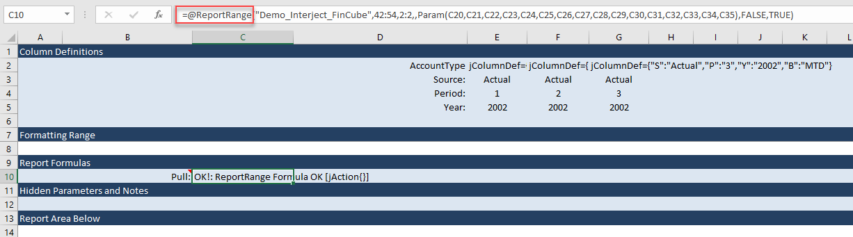
Now you are ready for the next step, changing the ReportRange() formula in C10 to a ReportVariable function.

Converting ReportRange() to ReportVariable()

Now you will convert ReportRange() to ReportVariable() to populate each financial group section in the row format. An automatic conversion is not available yet but changing the formula can be done quickly with the following steps.

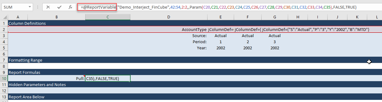
Step 1: Select the cell C10 and look at the Formula Bar. The ReportRange() formula needs to change to ReportVariable(). Change the wording as illustrated below.

Before:

After:

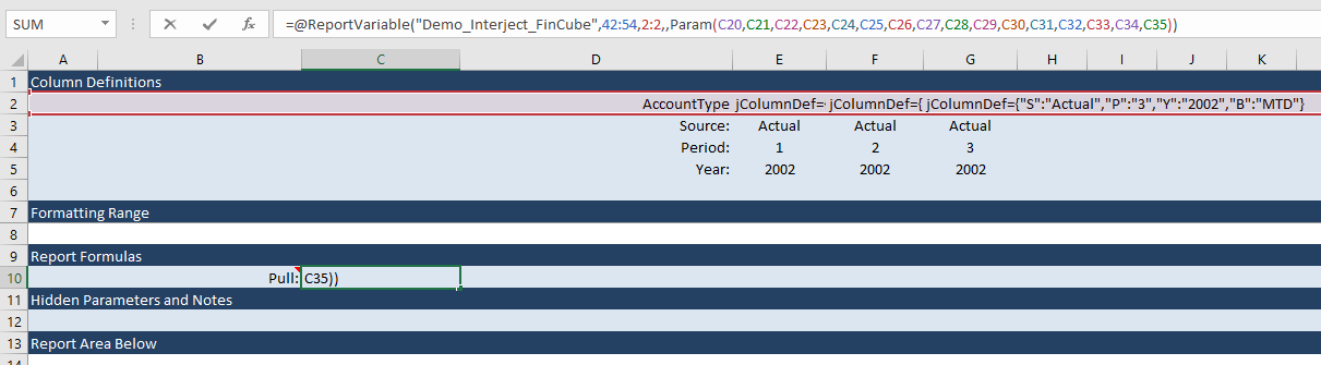
Step 2: Next remove the last two arguments. Remove ,FALSE,TRUE that is at the end, but keep the ) at the end. It should look like the below screenshot when removed. Noticed the formula will end with two parenthesis, like )).

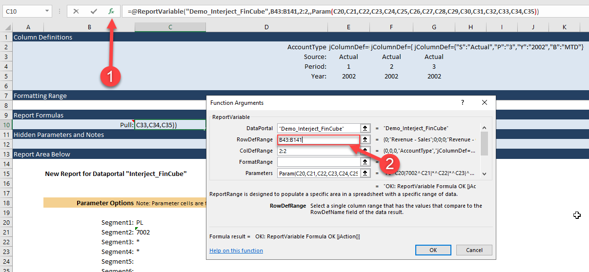
Step 3: With the above two edits, the formula is converted and you can click the fx button to review the arguments. The only argument that still must change is RowDefRange. This must change to select the list of Account Types that were setup in column B in previous steps. In the below example, you see that the first Account Type started at B44. Go up one row above and include at least one row below the last Account Type and enter B43:B141 into the RowDefRange argument.

Step 4: Before you can pull the ReportVariable() data for the first time, edit the Column Definitions. You last left Column Definitions with only AccountType in D2 along with 3 amount columns. This pulls a unique list of Account Types with their corresponding amounts. However, for this financial report you need to see account level detail in each Account Type subtotal section. Change D2 to Segment1. As noted earlier Segment1 relates to a general ledger account for this demonstration.

Next, you must type AccountType in cell B2. This is purposefully above the RowDefRange you defined a moment ago. By placing this column name in that column, Interject will expect that column value to define how data rows are included in each of the subtotal sections.

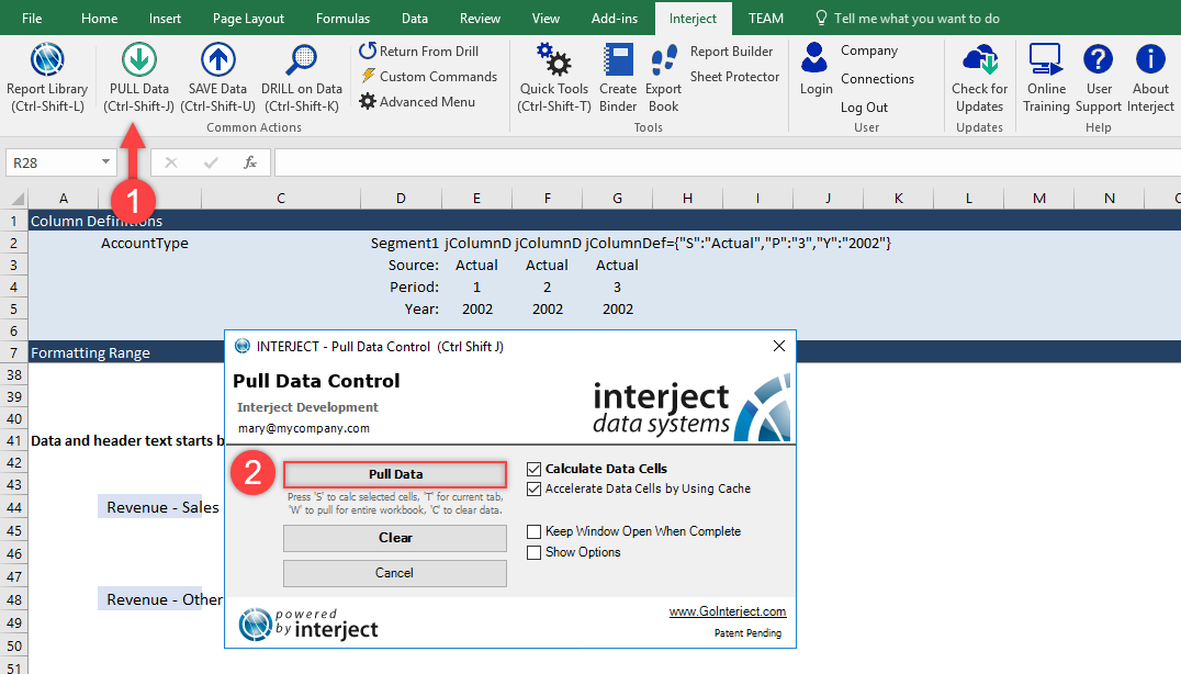
Step 5: Now you are ready to pull the data. Use the Pull Data menu item to pull the data.

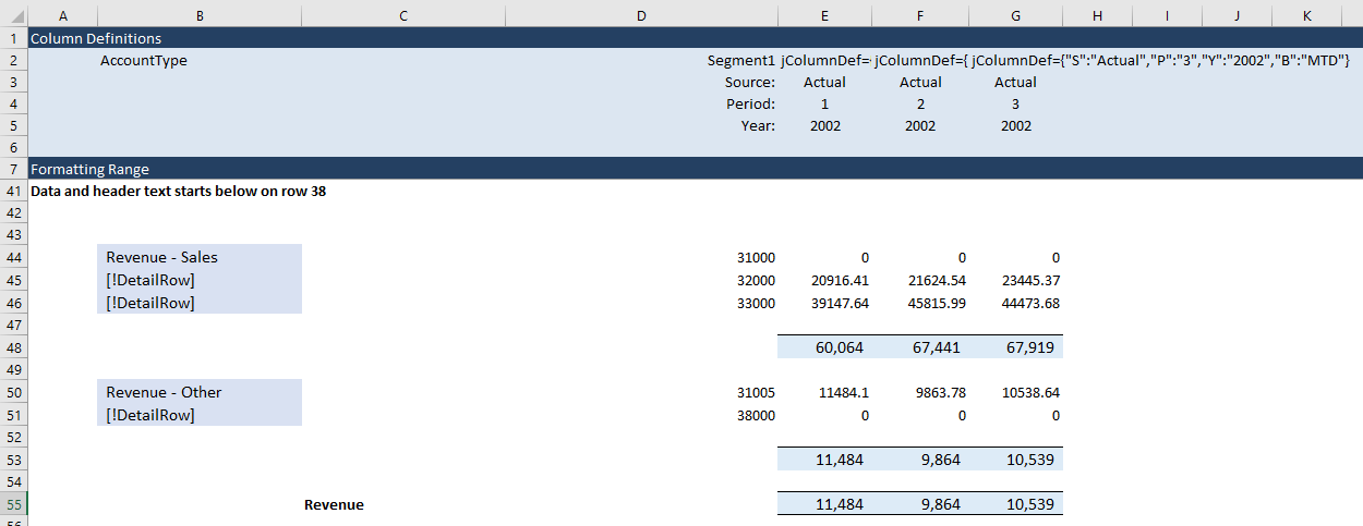
The data presented should look similar to the below screenshot. The Revenue - Sales section has three accounts listed and the totals are shown in row 48. There are new values in column B shown as [!DetailRow]. These values appear for each new row that is automatically added. These extra values will be deleted if you clear the data.

Final Formatting

Once the report is functioning and each subtotal section is expanding with data as needed, the rest of the work is simply spreadsheet work. There are a few key points to explain to make the spreadsheet work go a little faster.

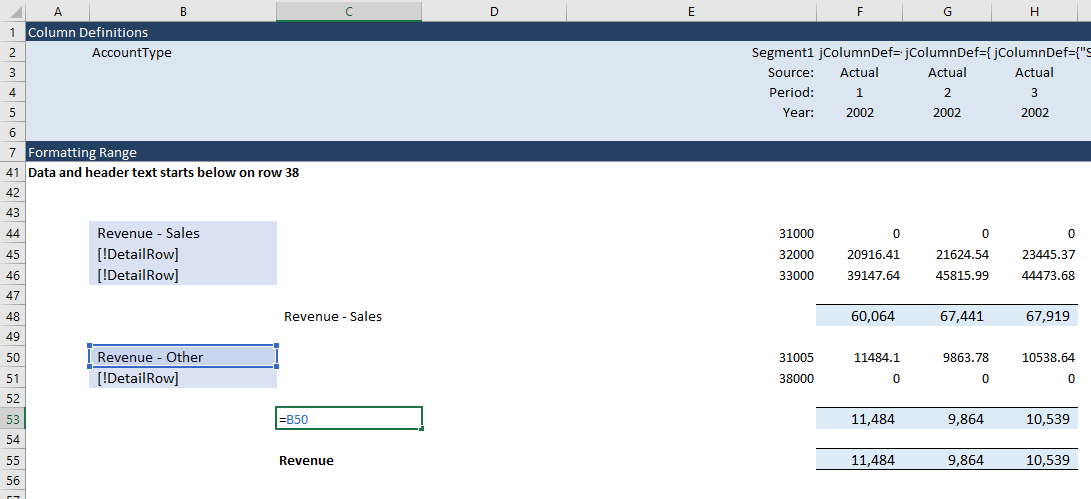
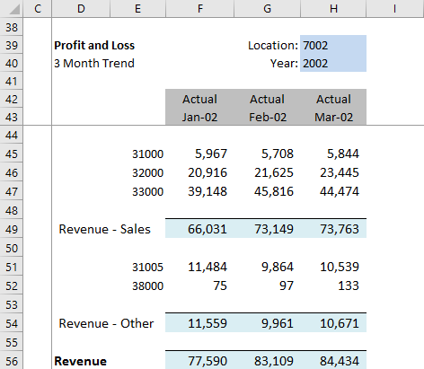
Point 1: Subtotal descriptions: The Row Definition in column B is typically hidden from view in the final report. You can insert a new column in between columns C and D to make room for the definition and you will add a formula in column D to equal the Account Type so it can show. In some cases, you could type in a more appropriate section name if not equal to the Row Definition value for that section.

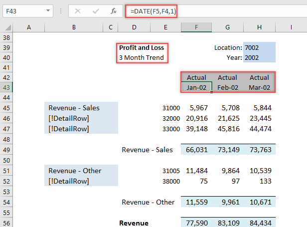
Point 2: Filters/Headers/Titles: In this screenshot there is an illustration of some of the small formatting options that help. For the column headers, they can link to the Column Definitions. The Actual value simply references the Source above on row 3. The months like Jan-02 uses the Date() function that points to the year and month in row 4 and 5. And do not forget to put a title on the top left.

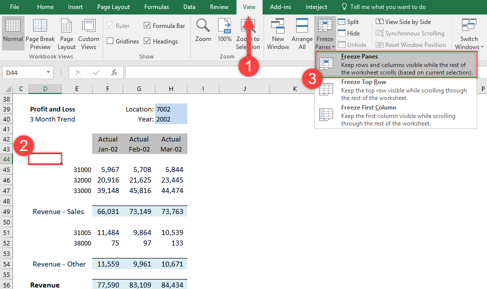
Point 3: Freezing panes: For ReportVariable() reports that have Row Definitions, you have to freeze the panes both vertically and horizontally. It helps to insert a new spacer column and keep the width narrow as shown below in column C. When freezing panes, you need to be sure to set the pane on the right of the spacer column. If set right next to the left side of the spreadsheet, the freeze panes will not lock horizontally.

Point 4: The Leftovers section: An important element for financial reports is a means to check the totals. Interject provides a method to ensure all data is presented. Including a Leftovers section at the bottom of the report will help provide assurance if all data did not get assigned to any subtotal section in the report created.

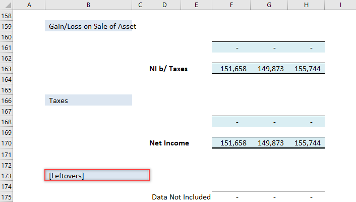
This concludes the exercise on creating a financial statement with Interject. There are still many more details to share but this will provide a foundation to get started. Once all the steps have been followed the report will look as below.

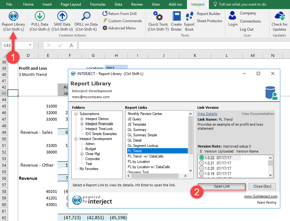
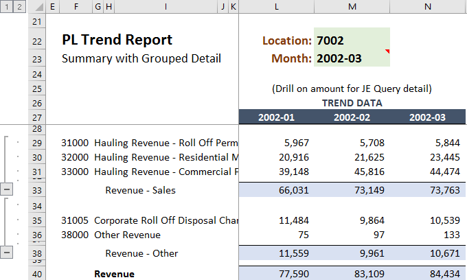
Next, you can open up the PL trend to see how the created report compares. Do this by selecting the Report Library and selecting PL Trend.

Then pull the data, set the location to 7002, and the date to 2002-03. Then select the 2 in the upper left corner to expand the groupings.

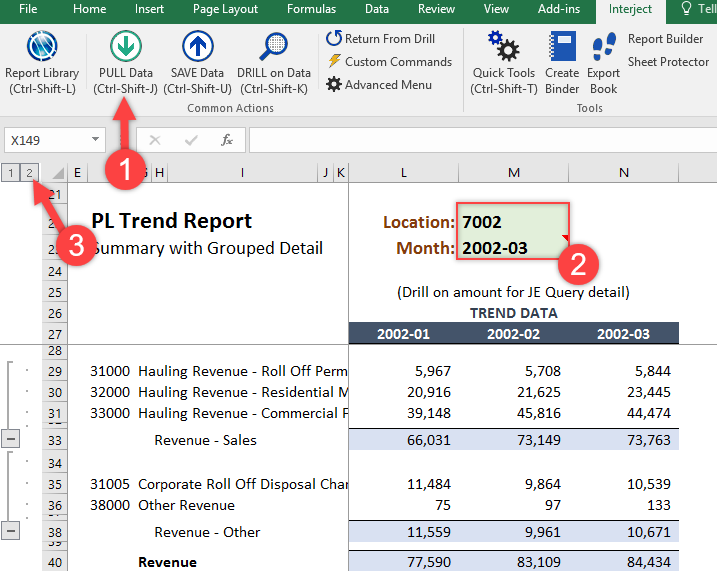
Ta-Da! After comparing the reports you can notice that, besides some formatting differences, the reports are the same.

Finally, clear the report, refreeze the panes, and upload it to the Report Library.

Do not upload this file to the Report Library if you are following the Training Labs. You may save the file locally, however, if you want to keep a local copy.