Create: Customer Aging Detail Report

Overview

This example uses the Customer Aging demo to show the creation of a Customer Aging Detail report that will have variable customer subtotaled sections, each having their respective invoice detail. You will use both the ReportRange() and ReportVariable() formulas to create the output.

If you are following the Training Labs, this is Lab 3.6. Note: The Report Library at Training Labs for this lab will be blank as you are creating a report from a new blank Excel sheet.

Building the Report

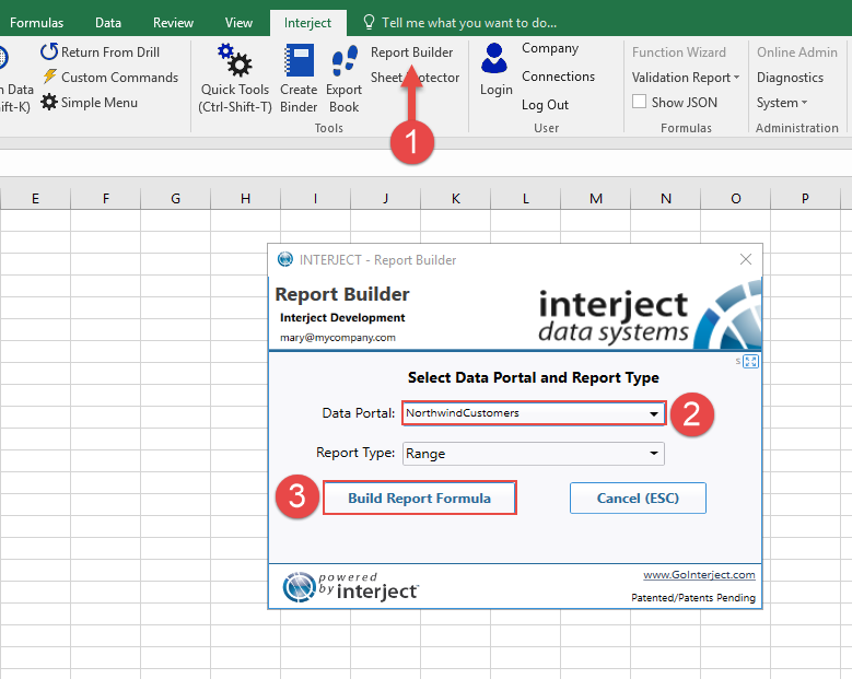
Step 1: You will begin by using Interject's Report Builder to make a template for the report. Select NorthwindCustomers Data Portal and choose Build Report Formula to build the report.

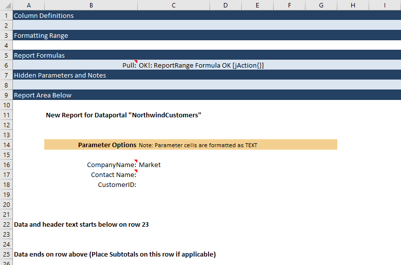
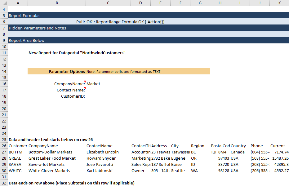
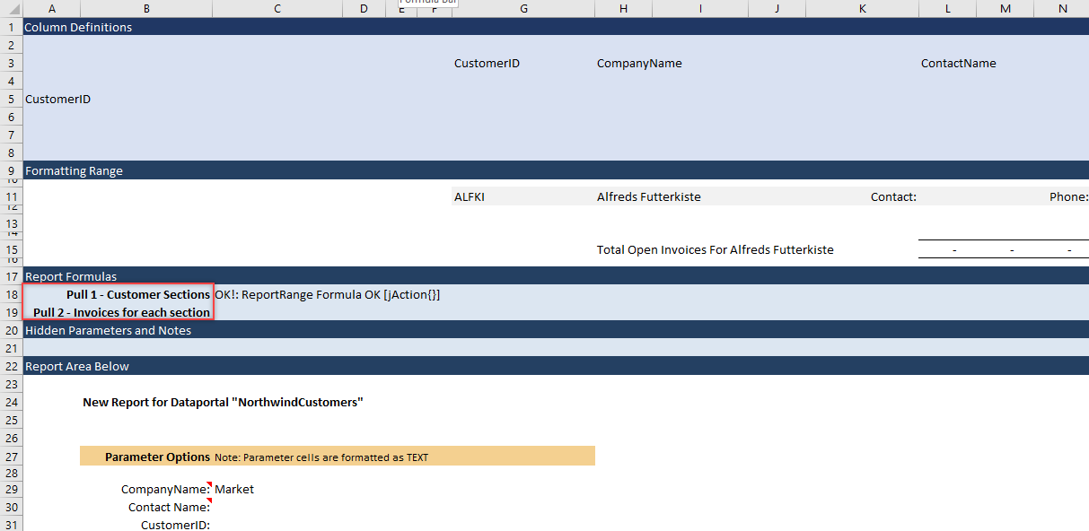
When the template is complete, it should look like the one below.

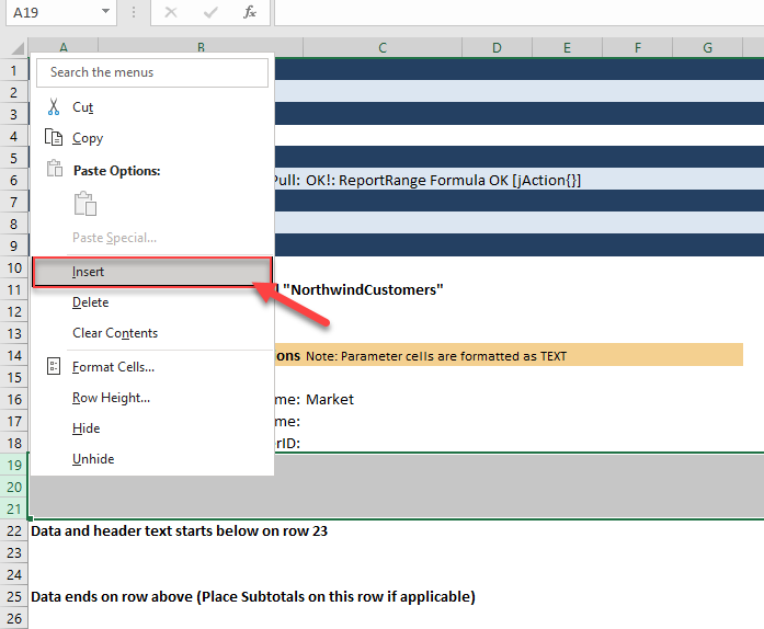
Step 2: Add 3 rows above row 25. Highlight rows 19-21 and rick-click on row 19 and click Insert.

ReportRange()

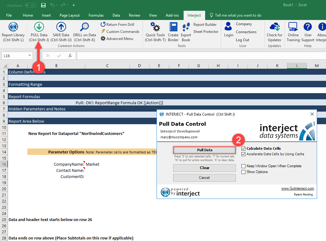
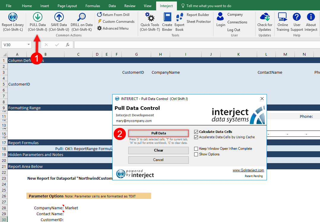
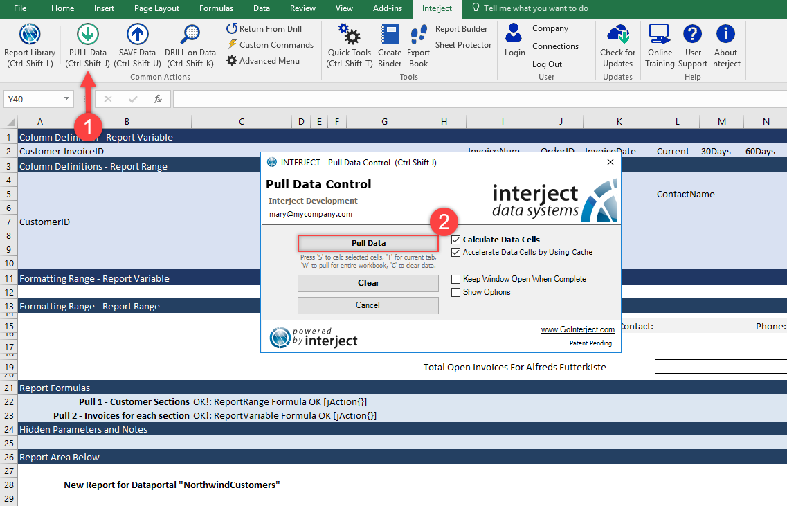
Step 1: You can select Pull Data to see which columns are available. Since the ReportRange() function does not have a Column Definition defined, it should show all the columns with their column names.

After you pull the report it will look similar to the one below.

Step 2: Now that you have pulled the data, you can copy the headers you want into the column definitions row. Do this by holding Ctrl and clicking CustomerID, CompanyName, ContactName, and Phone. Then copy them and paste the values into cell A2. The below animated GIF illustrates the copy process.

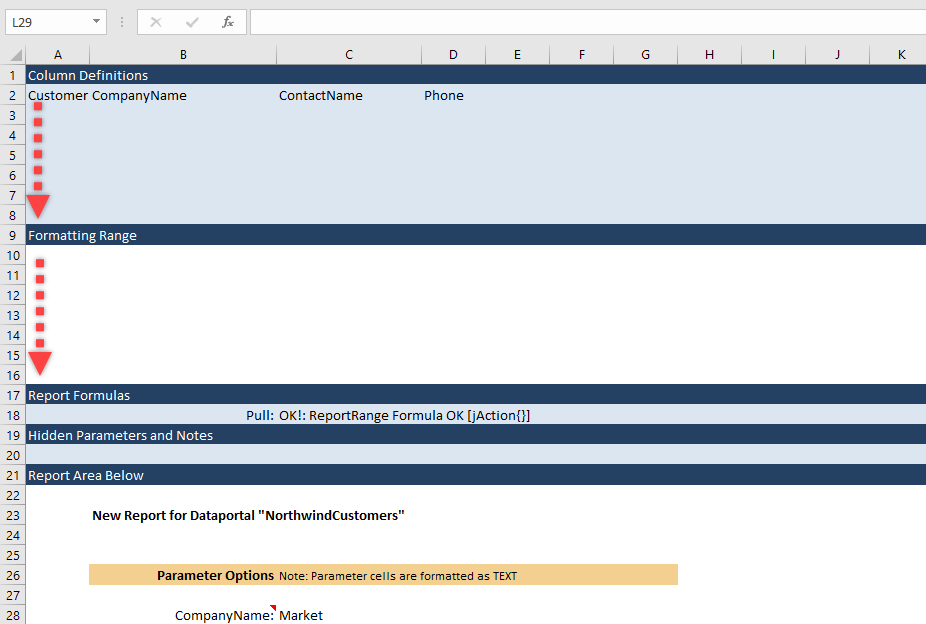
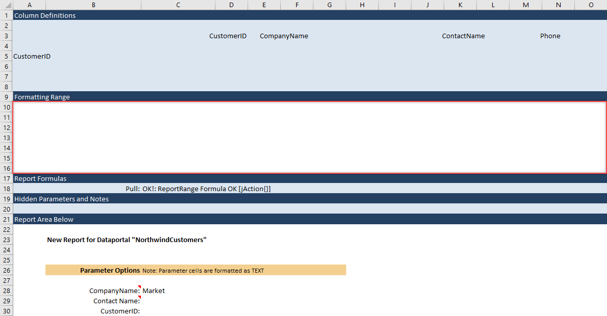
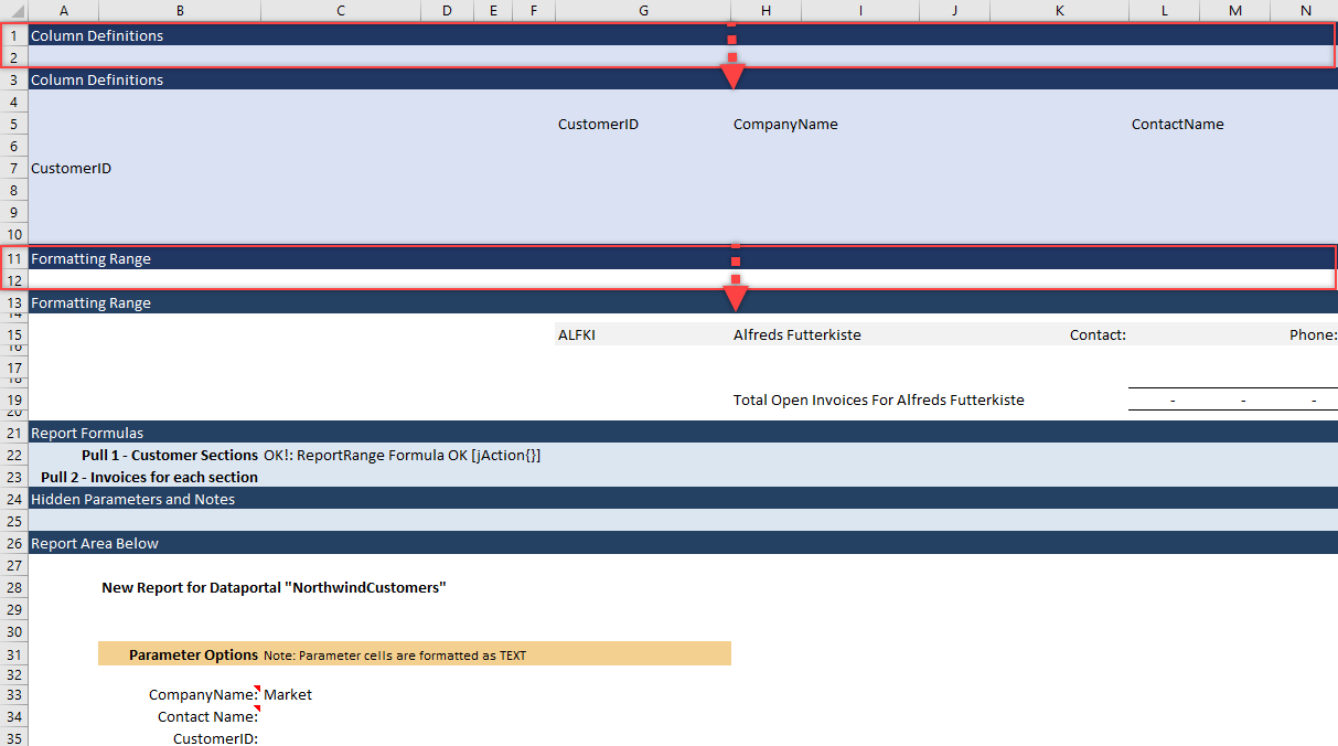
Step 3: For this report, you need to use the multi-row feature illustrated in a previous example. This will be the complete subtotal section that will be repeated for every customer shown. You will insert 6 rows under the Column Definitions row 2 and insert 6 rows under the Formatting Range row 10. This will give you room to format the report. Each section should have 7 rows beneath it, as shown below.

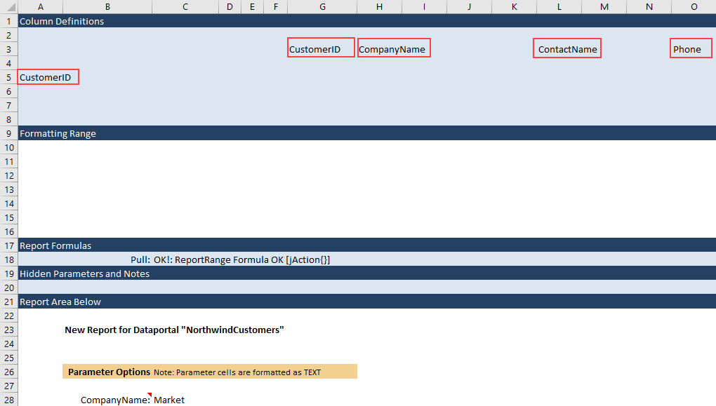
Step 4: Now you will move the Column Definition values into the correct positions. Move CustomerID to cell A5, another copy of CustomerID to cell G3, CompanyName to cell H3, ContactName to L3, and Phone to O3. You can also format the width of the columns to best fit the report. Match the following screenshot with the column widths.

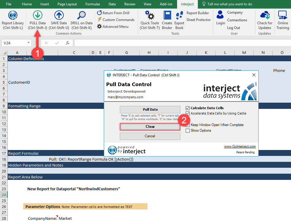
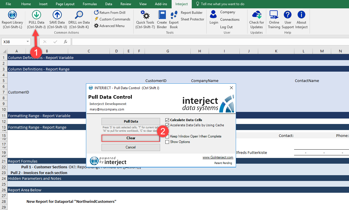
Step 5: Before you setup the Column Definitions in the ReportRange() function, it is best to clear the report so the previously pulled data is erased. Use the Pull Data menu item to select the Clear button as illustrated below.

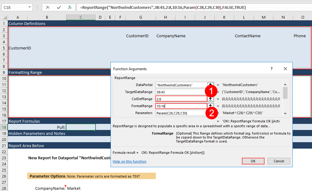
Step 6: Next, edit the ReportRange() formula. To access the formula you will select the cell C18 and click fx to bring up the Function Wizard.

Now add the ColDefRange and the FormatRange. Type 2:8 for the ColDefRange and 10:16 for the FormatRange as shown below. Notice these are encompassing all 7 rows you have for each section.

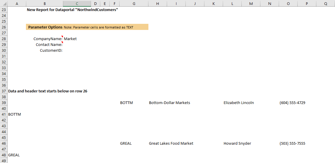
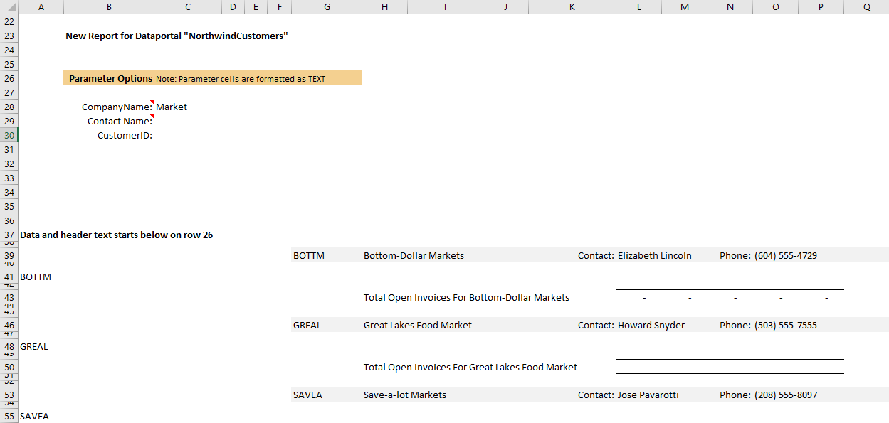
Step 7: If you re-pull the data, the multi-row format will be repeated for every customer.

As seen in the following screenshot, you have 7 rows for each customer. It is not formatted yet, so it will not be clear which this is used for. But you can keep moving on.

Step 8: You can begin setting up the Formatting Range.

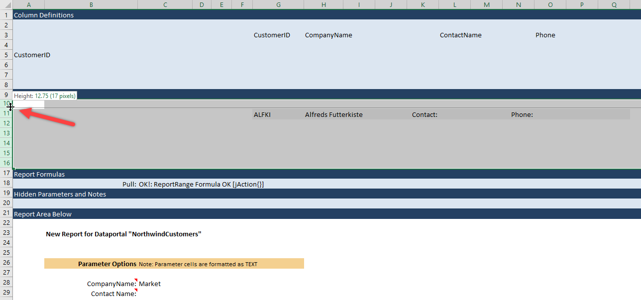
Give row 10,12,14, and 16 heights of 6.75. The image below illustrates how to drag the row height to get close to 6.75. You can also type in example data in G11, H11. In K11 you can type in a label Contact : and Phone: in N11. Format both of these to be right-aligned.

Step 9: Now you need to create a formula that will total all of the detail that will later be populated between row 13 and 14. To create a total, type =SUBTOTAL(9,L13:L14) in L15. In cell H15 you will type ="Total Open Invoices For " & H11. H11 represents the name of the customer, and by linking it to H11, the subtotal line will note the customer name again.

After that, you will copy the formula put in cell L15 to cell M15, N15, O15, and P15. These subtotals will be used for the aging buckets that will be setup later in this page. See the example below and adjust the formatting to match.

Step 10: Re-pull the data to make sure it is formatted correctly.

The formatting has been copied down to the rest of the report and there are subtotal sections. Now you need to populate the section detail with the customer invoice detail.

ReportVariable()

Step 1: In the Report Formula Section, add a new row under row 18.

Step 2: Rename the first pull to Pull 1 - Customer Sections (in cell B18) in order to keep track of the report formulas. In cell B19 type in Pull 2 - Invoices for each section. The new ReportVariable() will be added to C19 shortly.

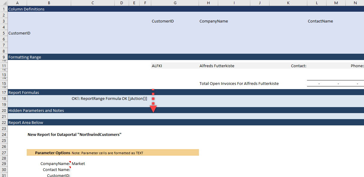
Step 3: Because you are adding a new Report Formula, you need a new Column Definition and Formatting Range. The illustration below shows two additional sections added. Please update to match.

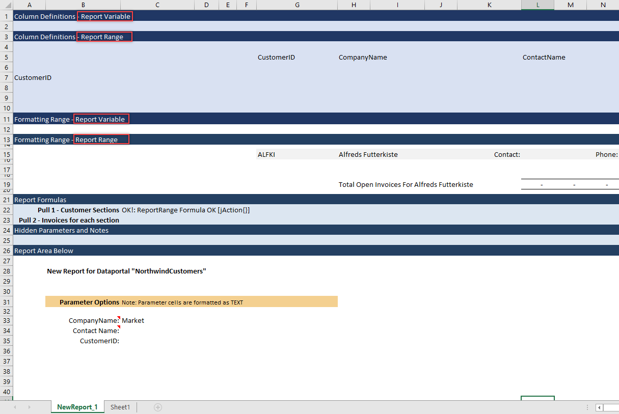
Step 4: Since you have ranges and definitions for both of the formulas, you will rename them so you know which formulas they specify. Please update cells A1, A3, A11, and A13 to match the following text.

Step 5: Now you will clear the data to prepare for creating the new formula.

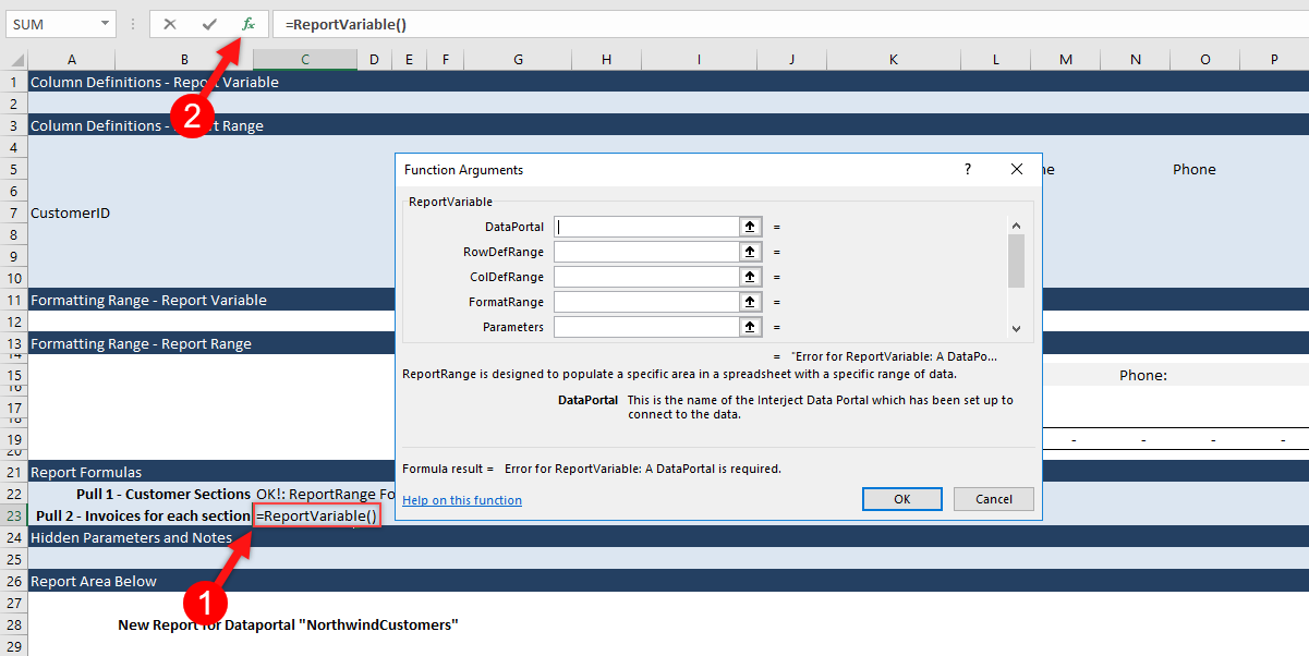
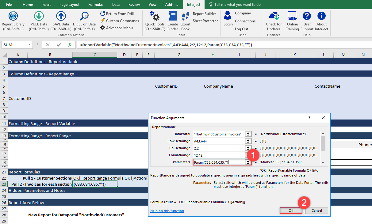
Step 6: To define the second formula, add =ReportVariable() to cell C23 and click the fx button. The placement of this formula matters, since you want it to run after the ReportRange(). The ReportRange() will be pulled first to provide the list of customer sections, and then the ReportVariable() will populate the invoices for each section.

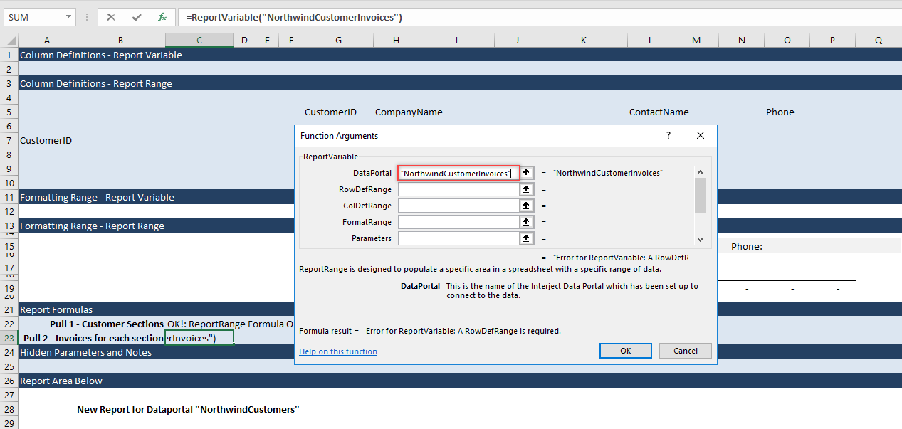
Step 7: Using the Function Wizard, add NorthwindCustomerInvoices as the Data Portal.

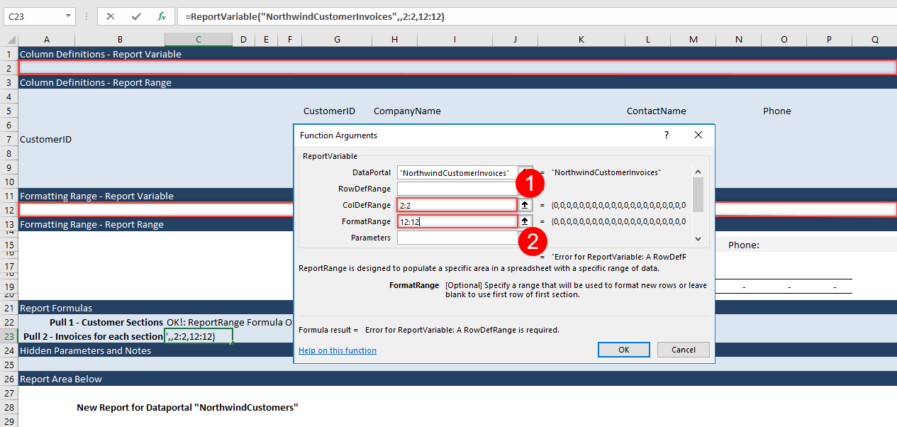
Step 8: Next, you will specify the new Column Definition and Formatting Range. Type 2:2 into ColDefRange and 12:12 into FormatRange.

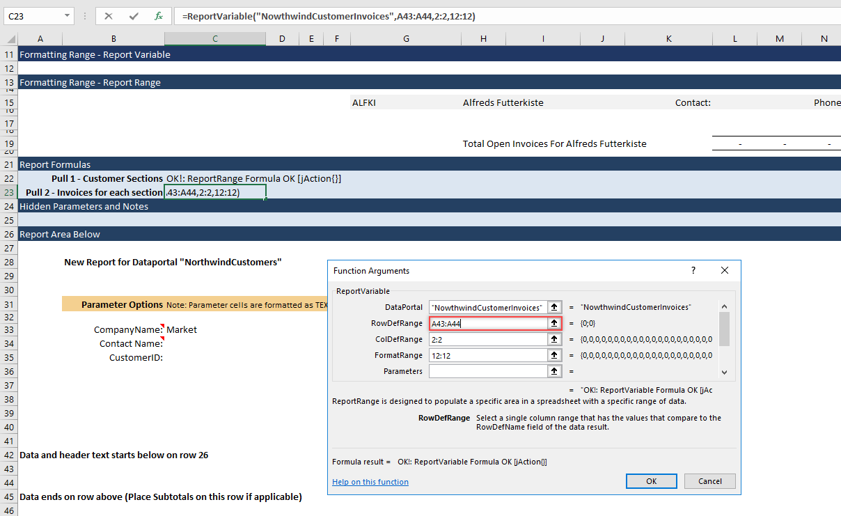
Step 9: With a ReportVariable, a RowDefRange is required, since it marks what data is to be included in each section. Type A43:A44 into the RowDefRange. You will be placing the CustomerID in column A shortly.

Step 10: Now type Param(C33,C34,C35,"") to establish the parameters for the formula that match the previous ReportRange(). Both Report Formulas are setup to use the same filters. Click OK to finish.

Step 11: Before the pull, you need to specify the columns for the invoices that will be included in the detail section. Type CustomerID in cell A2, InvoiceID in cell B2, InvoiceNum in cell I2, OrderID in cell J2, InvoiceDate in cell K2, Current in cell L2, 30Days in cell M2, 60Days in cell N2, 90Days in O2, ExpectedDate in R2, and Note in T2. Please note that the screenshot below may not show all the characters that need to be typed. Please double check with the last sentence.

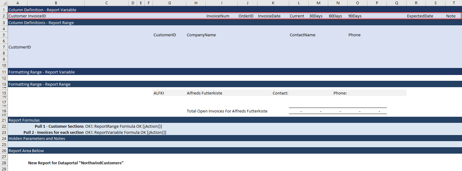
Step 12: Once completed, re-pull the data.

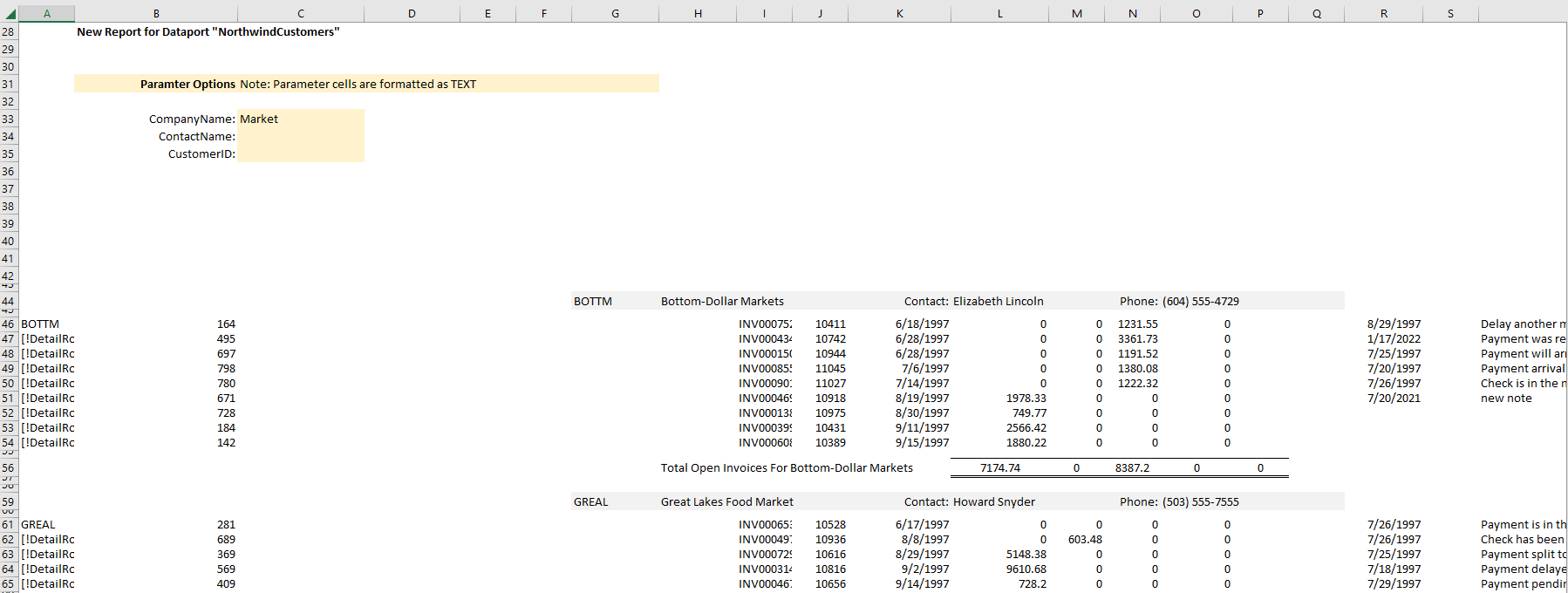
After pulling the report you now have invoice detail in each section.

ReportDefaults()

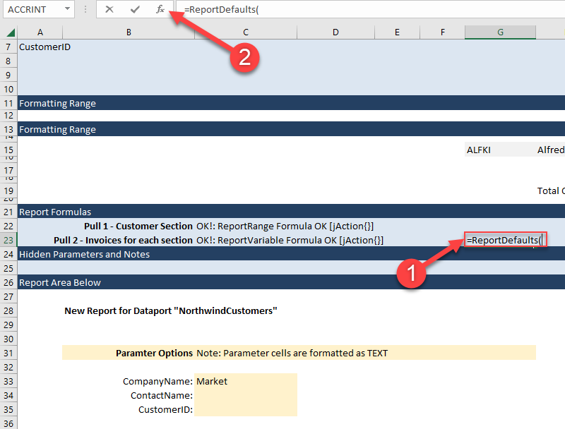
Step 1: The parameters in C33:C36 are not cleared after clearing the data. You can setup a ReportDefaults() formula to have these cleared after you clear the data. ReportDefaults is an event function, which means it triggers on a particular Interject event. Click on cell G23 and enter =ReportDefaults() and click on the Function Wizard button.

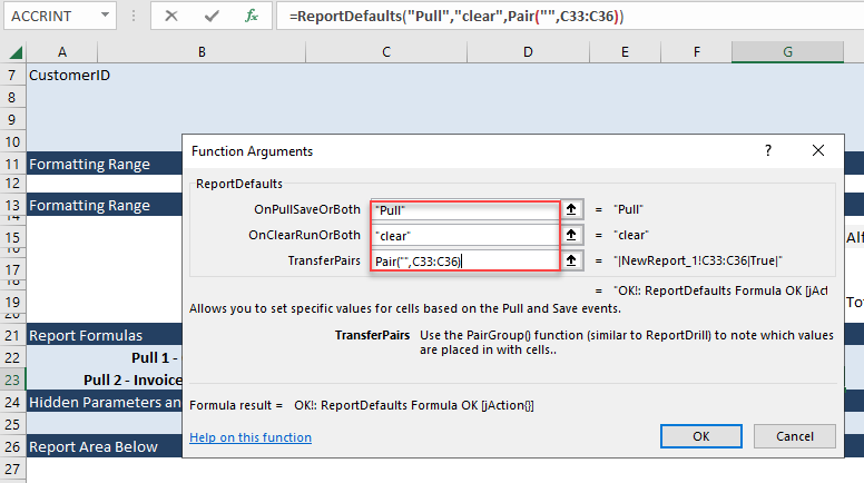
Step 2: Enter Pull for OnPullSaveOrBoth field, clear for OnClearRunOrBoth, and Pair("",C33:C36) for TransferPairs. This will transfer "" into cells C33:C36 after a Pull-Clear event.

Step 3: Clear the report.

Notice the parameters are reset.

Formatting the Report

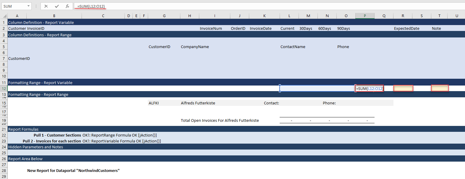
Step 1: You can go a step further and setup the formatting for the invoice detail and add a subtotal formula in row 12.

Type =SUM(L12:O12) into cell P12 to add the formula for total. You will also change the color on cell R12 and T12.

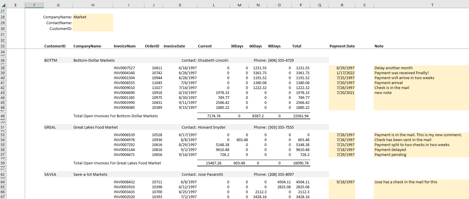
Step 2: After you add some headers–and move some cells, freeze panes, and formatting–the final product will look like this.

Finally, clear the report, refreeze the panes, and upload it to the Report Library.

Do not upload this file to the Report Library if you are following the Training Labs. You may save the file locally, however, if you want to keep a local copy.