Create: Customer Aging Report

Overview

In this page you will see the process of building a Customer Aging report from scratch to better understand reports and also get a clearer illustration of the Interject ReportRange() data function.

If you are following the Training Labs, this is Lab 3.1. Note: The Report Library at Training Labs for this lab will be blank as you are creating a report from a new blank Excel sheet.

Building the Report

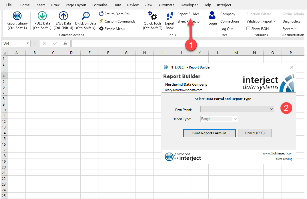
Step 1: This process begins with the Interject Report Builder . Open the Report Build as illustrated below. There is a drop down list of Dataportals that can be chosen . An Interject Data Portal is a pre-configured data query that is setup so spreadsheet users can easily direct data into their own spreadsheet reports. Data Portals can be setup to access databases or cloud data and are either setup by Interject developers or the IT team.

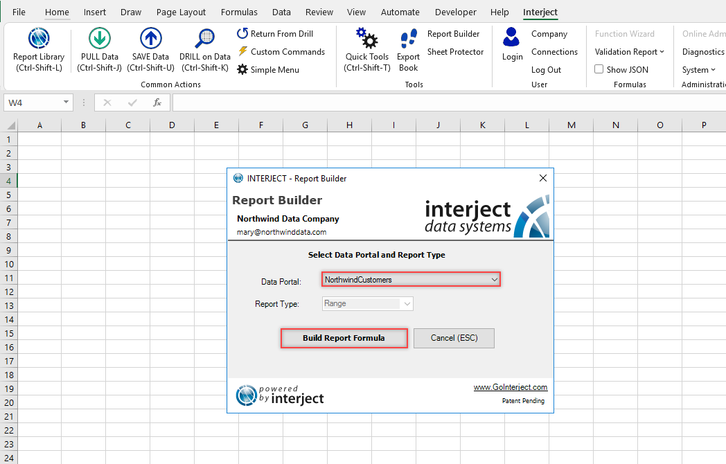
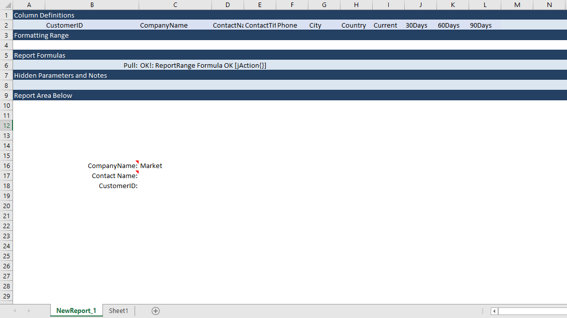
Step 2: For this Customer Aging report, use the NorthwindCustomers Data Portal. Once chosen, click the Build Report Formula button.

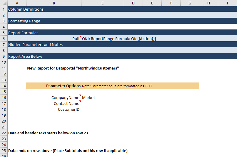
A new sheet should be added that looks like the screenshot below. Now the report is ready for further customization.

Getting Started

Step 1: Begin by putting the filter value Market in C16 so you can limit the data pulled to just a few records that have a Company Name that contains the word Market.

Next, use the Pull Data menu item.

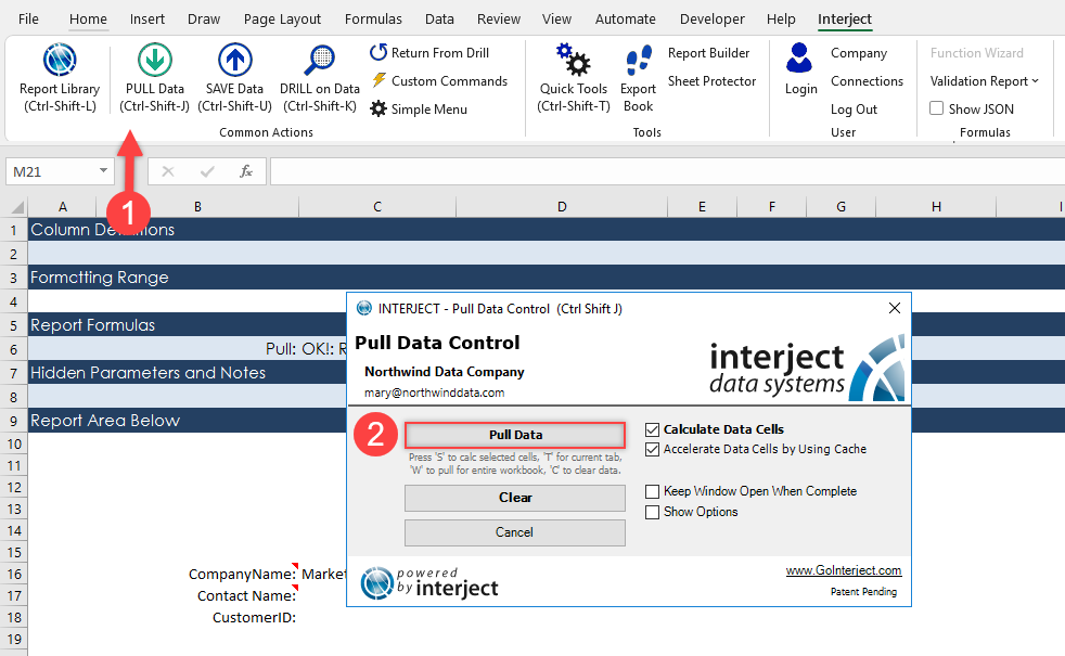
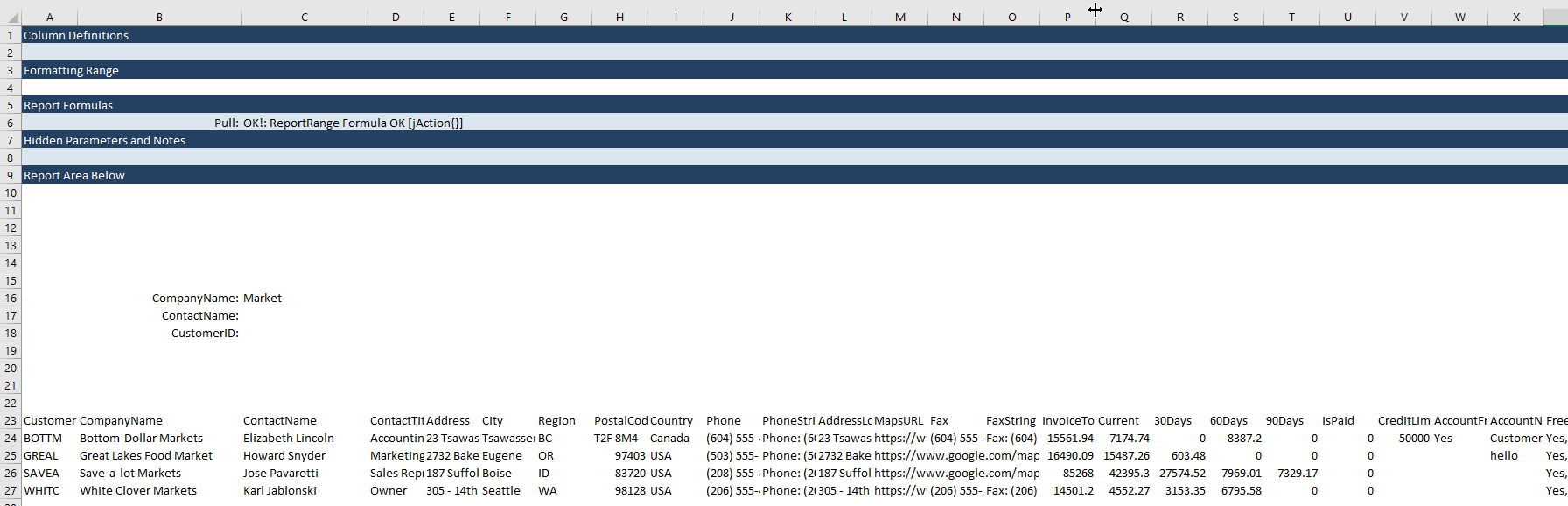
You can see below, that all the columns available in the Data Portal will be shown by default with the column names on the first row.

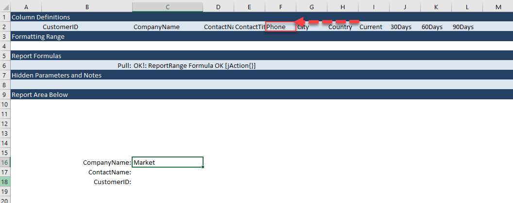
Step 2: Select a few columns for our report by copying a few of the column names to the Column Definition area on row 2. Follow the animated GIF below to multi-select CustomerID, CompanyName, ContactName, ContactTitle, City, Country, Phone, 30Days, 60Days, and 90Days. You can select them all individually while holding the Ctrl key. Then you can copy and paste the values all at once in cell B2.

Step 3: Now that you have the columns, move the Phone column title to column F instead of H. First select the entire column H. Then hold the Shift key and hover your cursor over the left border of Column H. Left-drag the column left until the pop-up says "F:F" and then let go.

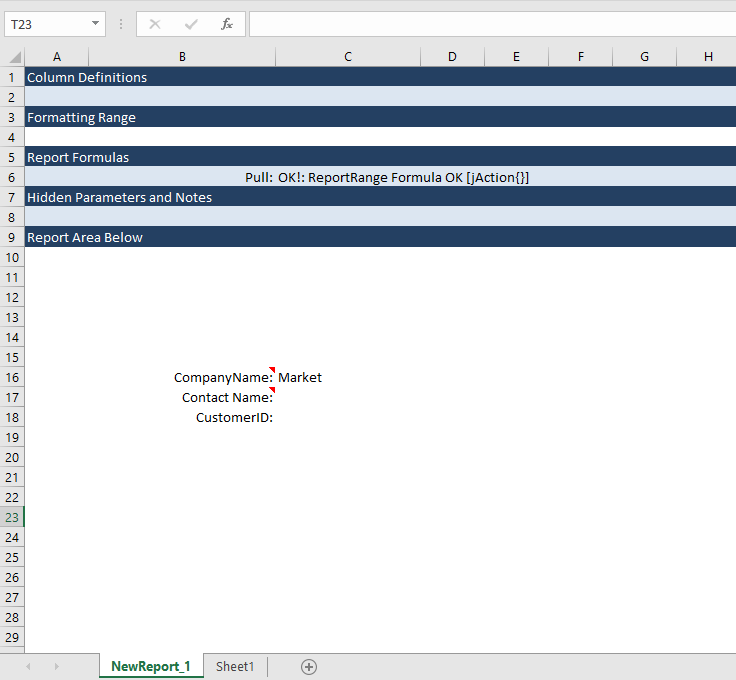
Step 4: Now that the Column Definitions are set, clear the report for the next step.

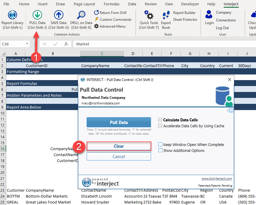
The cleared report should look like the screenshot below.

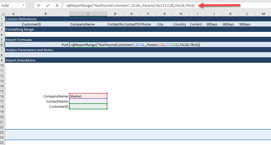
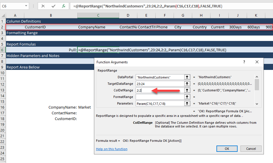
Step 5: Now set up the ReportRange() formula to look to the Column Definition area that was just set. Select cell C6.

Step 6: Click the fx button as noted below to open the Function Wizard and add a ColDefRange. The ColDefRange argument should be empty at first.

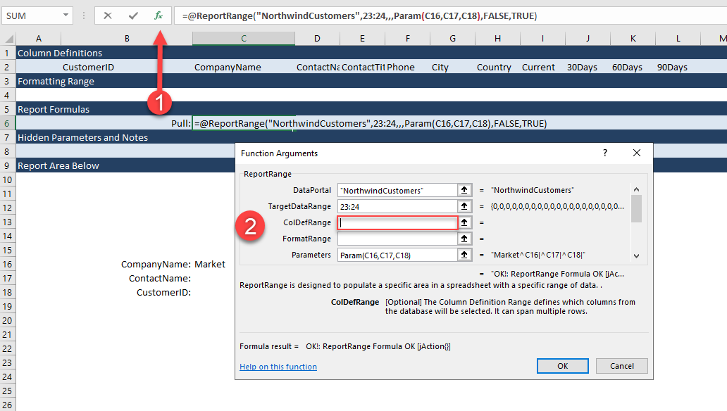
For this report, you will set the ColDefRange to the entire second row, 2:2.

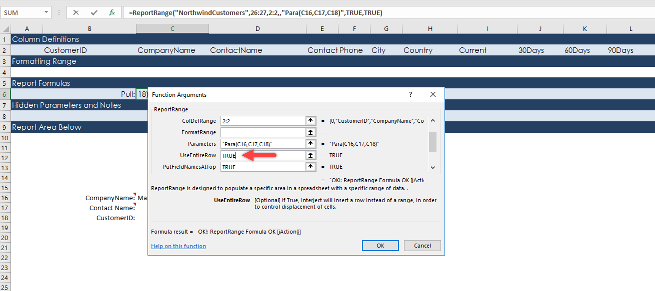
Step 7: Next, scroll down in the Function Wizard to view the UseEntireRow argument. Change from FALSE to TRUE. This is an optional step but is certainly a best practice.

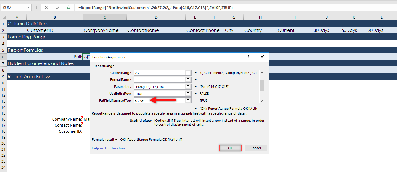
Step 8: Before closing the Function Arguments, continue to scroll down so you can change the PutFieldNamesAtTop argument from True to False. This is not required but is a good practice.

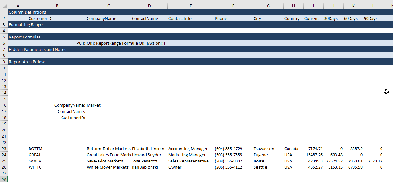
Step 9: When you re-pull the report, the selected 11 columns in the Column Definition should be the only columns showing.

Final Formatting

The data pulled should look like below.

Note : Although not illustrated in the below steps, you can save typing in the column labels for later. Copy the Column Definition values in B2:L2 and Paste Values in B22:L22. These are the labels you can customize for users to view.

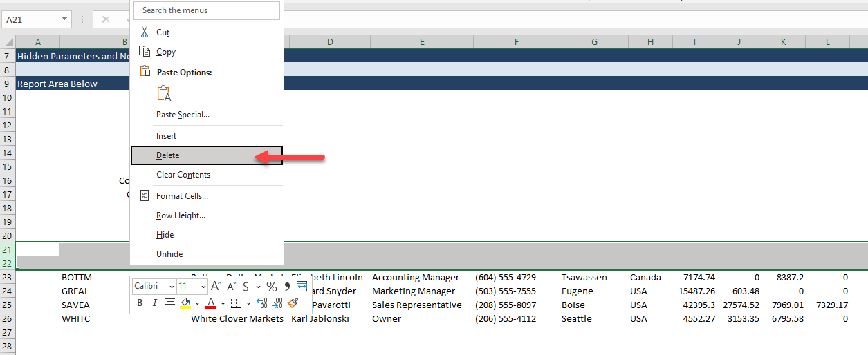
Do some quick formatting to clean up the report. Delete rows 21 through 22.

Setting up jFreezePanes

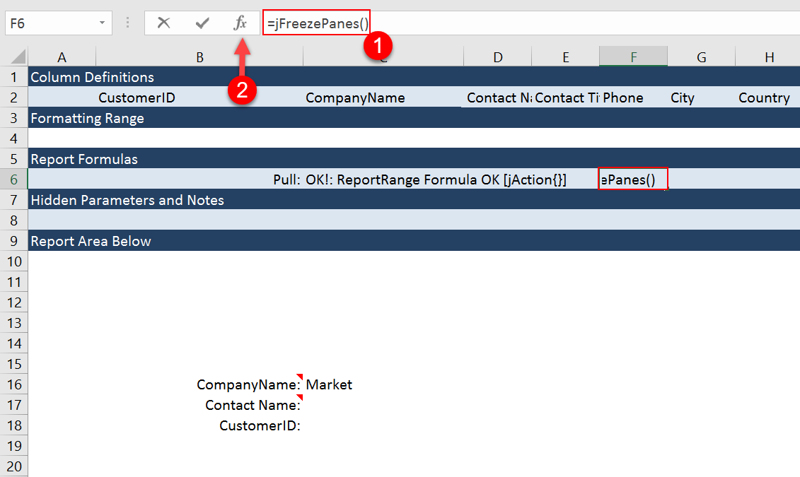
Next, you need to freeze the panes to hide the configuration area from the users. This can be done manually with the Excel menu item for freezing panes. But this is a good time to illustrate INTERJECT's jFreezePanes() feature. First, setup the jFreezePanes function by entering =jFreezePanes() in F6 and click the fx button.

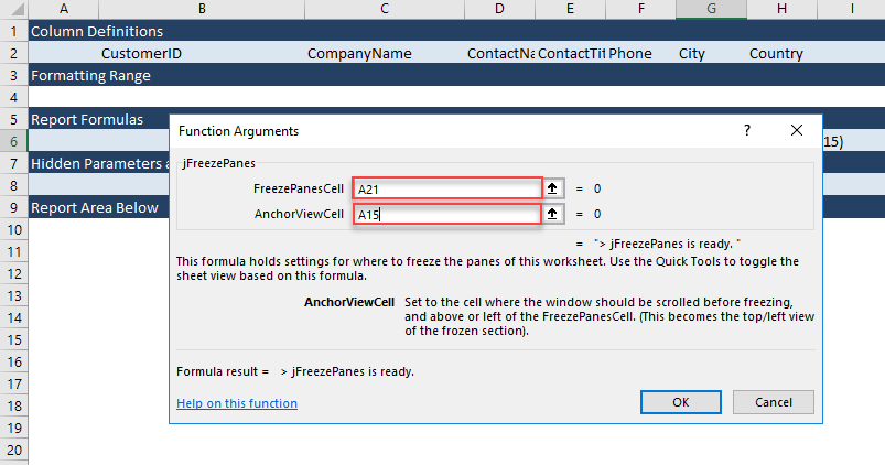
Step 1: In the FeezePanesCell argument, input A21 to mark that row as the top of the visible report. This sets the top of the report that will be visible to the user. For the AnchorViewCell argument, type in A15. This will set the row that will be frozen above A21, where you will place the column headers. Press OK.

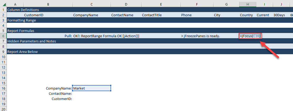
Now we will setup a jFocus() formula so that the cursor will be set to a particular cell after the panes are frozen. In this case, we want the active cell to be C16 after the freeze. Click on cell H6 and enter the formula =jFocus(C16).

Use the Quick Tools menu item in the INTERJECT Ribbon so you can easily freeze the panes using the jFreezePanes formula you just configured.

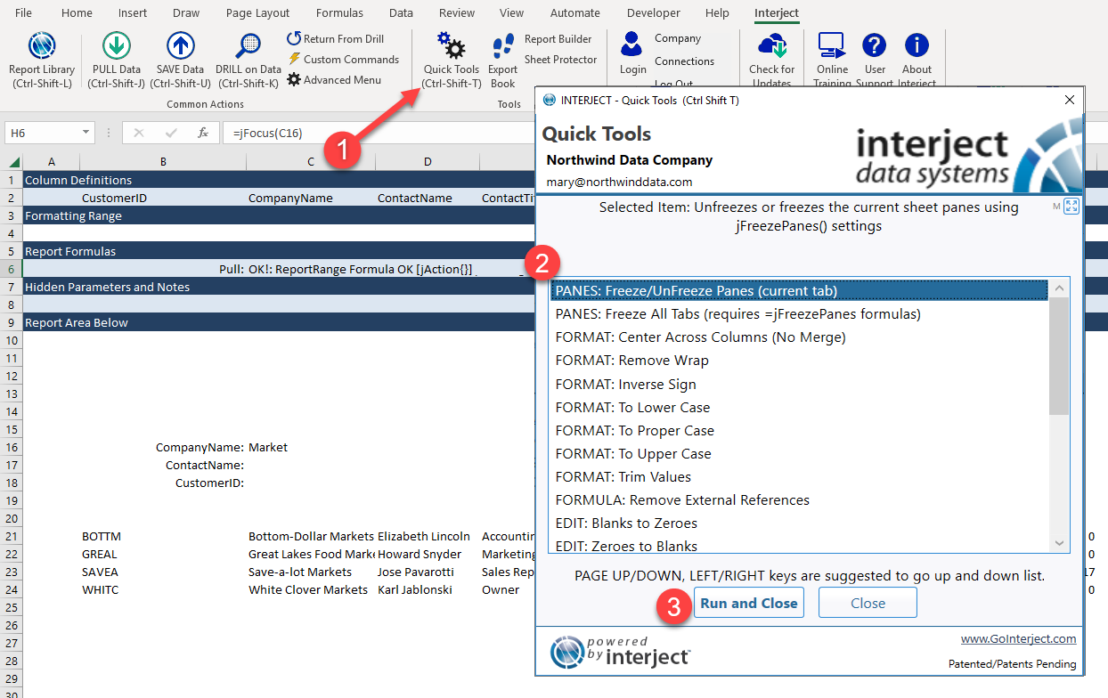
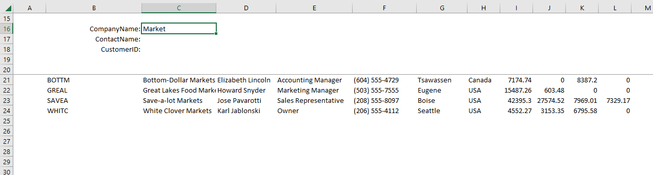
Step 2: The following should be the result after the panes are frozen.

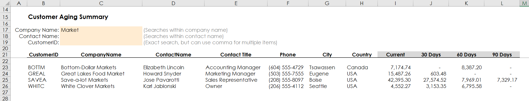
Step 3: This last view shows what the final report can look like when the report is complete. Add the column labels in row 20, the filter helper text in column D, and match the formatting. The data can be cleared and shared with other users as a search tool for customers.

Finally, clear the report, refreeze the panes, and upload it to the Report Library.

Do not upload this file to the Report Library if you are following the Training Labs. You may save the file locally, however, if you want to keep a local copy.