Advanced Row and Section Hiding

Overview

In this example of the ReportHideRowOrColumn() function, we will hide an entire section of a report based on the condition that the section is empty. You would typically use this in a report when data is pulled in with zero values. By hiding the zero value rows, and the entire section when all the rows within it are zero vale, the reporting area will be more usable.

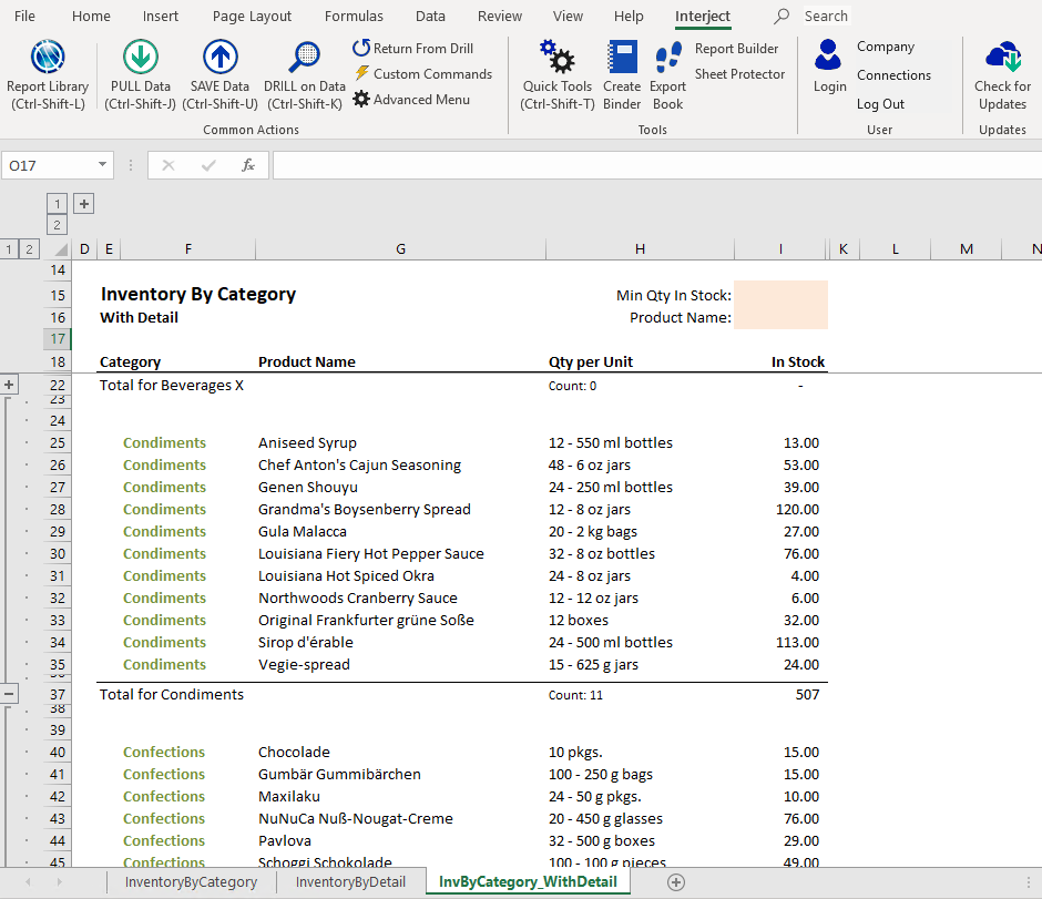
For this demo, find the Interject Inventory Demo in the Interject Demo folder within the Report Library. Once open, you'll use the InvByCategory_WithDetail tab.

If you are following the Training Labs, this report file can be found in the Report Library at Training Labs > Lab 5 Advanced Features > Lab 5.2 Advance Row and Section Hiding.

Hiding Rows

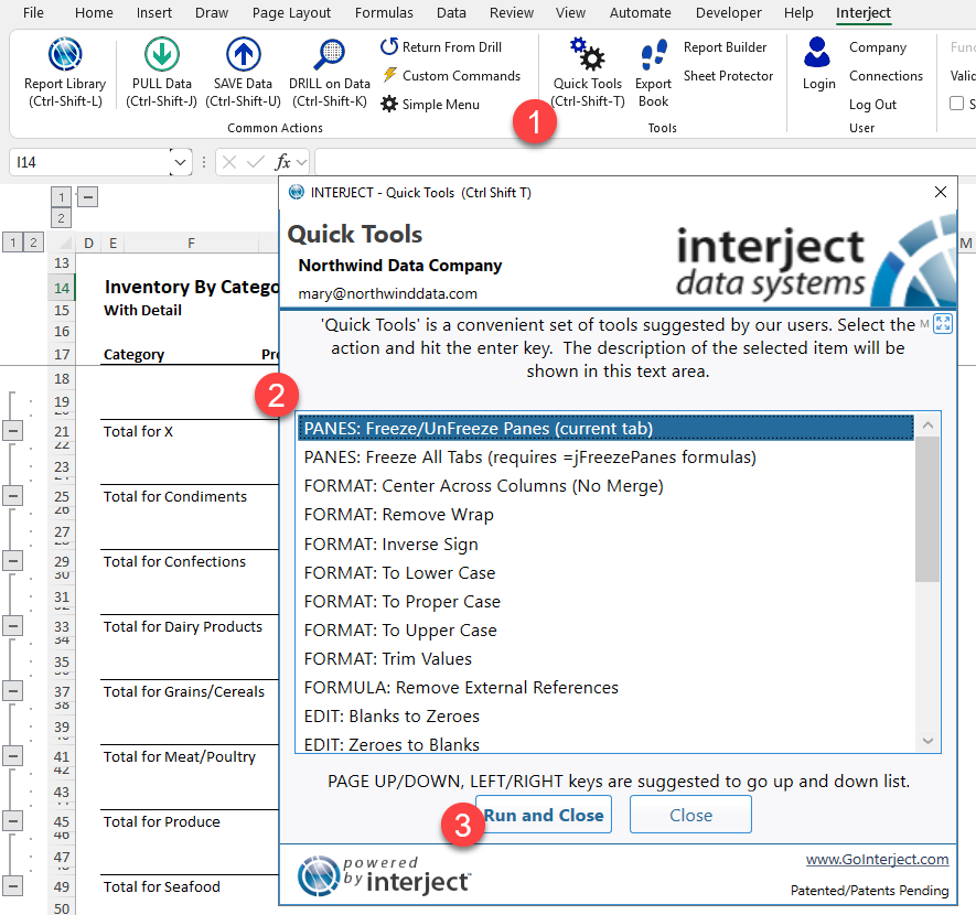
Step 1: Start by using the Quick Tools button in the ribbon menu and selecting Freeze/Unfreeze Panes.

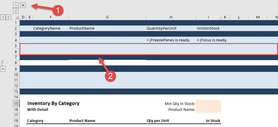
Step 2: Insert a row above row above row 6, so that there are 2 blank rows, and then expand the collapsed columns by clicking the plus sign in the upper left.

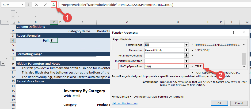
Step 3: Click into cell C4 and open the Function Wizard by clicking fx. Then scroll down in the Report Variable section of the wizard until you see UseTopSpacerRow, and type True into the empty field. Click OK.

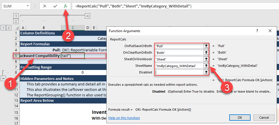
Step 4: In cell B5, type For Backward Compatibility:. Then, in cell C5 enter =ReportCalc() or double click it from the formula menu. Once it's entered, open the Function Wizard and input the following and click OK:

• OnPullSaveOrBoth: Pull
• OnClearRunOrBoth: Both
• SheetOrWorkbook: Sheet
• Disabled: Leave blank
• SheetName: InvByCategory_WithDetail

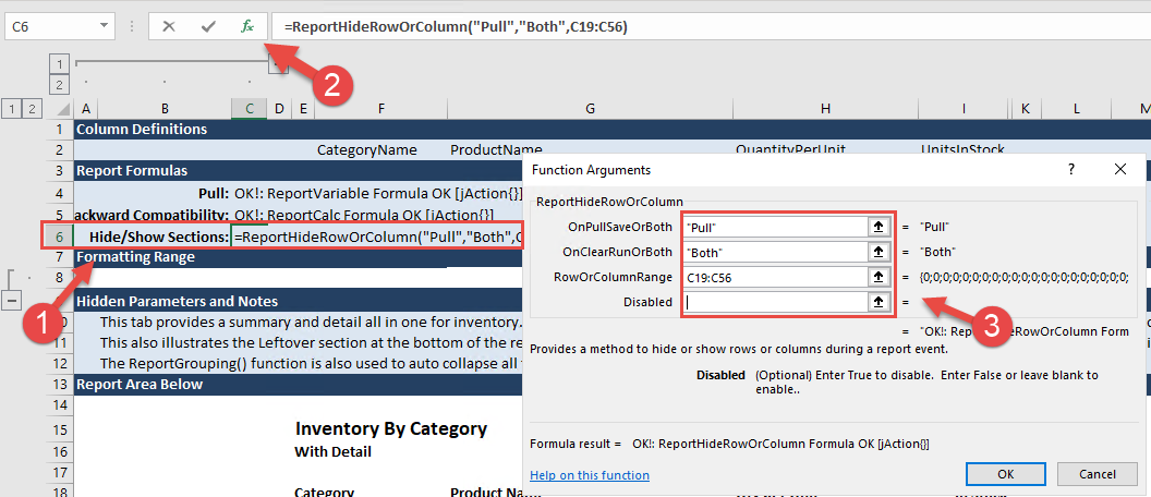
Step 5: In cell B6 type "Hide/Show Section:". In cell C6 type =ReportHideRowOrColumn() or begin typing and double click the formula from the menu. Next, open the Function Wizard by clicking fx, enter the following information and click OK:

• OnPullSaveOrBoth: Pull
• OnClearRunOrBoth: Both
• RowOrColumnRange: C19:C56
• Disabled: Leave blank

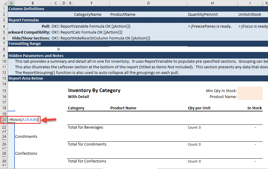
Step 6: In cell A20 enter =Rows(A19:A56).

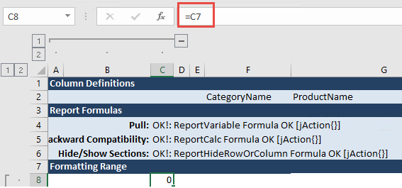
Step 7: In cell C8, enter =C7, to reference the cell above.

Step 8: Now, in cell C19 of the report area, write the formula =IF(AND(I22=0,$A$20<>38),"Hide","Show"). Write the formula =C19 in both C20 and C21.

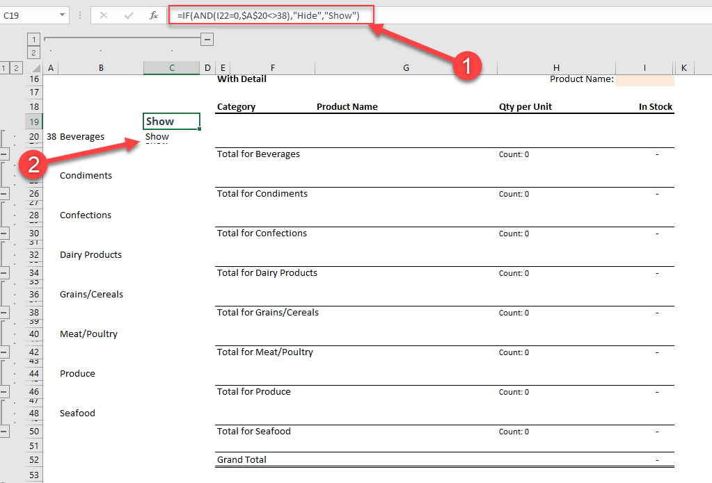
Step 9: Select cells C19:C21 and copy to the clipboard by pressing CTL-C. Navigate to cell C23 and paste the formulas by pressing CTL-V.

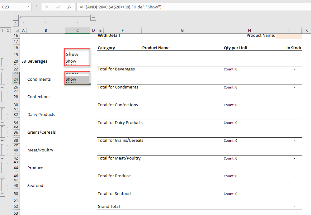
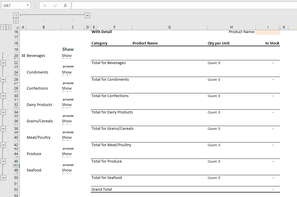
Continue to navigate to each category and paste the formulas in cells in C27, C31, C35, C39, C43, C47. The final result should look like the screenshot below.

Step 10: To test that the function and formulas are working correctly, click into cell B20, which contains the category name "Beverages" and add and "X". Now freeze the panes using the Quick Tools menu, hide the leftmost columns, and pull the report.

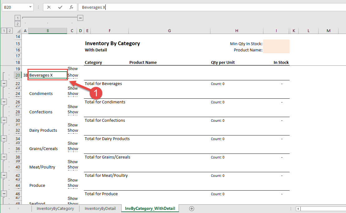
You should see that the empty category comes in collapsed, the other category detail is expanded, and the original "Beverages" category comes in at the bottom as "Items Not Included".