Create: Working with Pivot Tables

Overview

Pivot tables are a flexible and valuable tool for analyzing data in Excel. Interject makes it easier to scale and distribute pivot tables. In this walkthrough you will set up a pivot table based on an Interject report. There are a couple advantages to combining Interject with pivot tables. It provides the ability to build security into pivot table reports, users only see data relative to their credentials. Also, by allowing filters that are used at the database level, the amount of data in a user's pivot table is limited to data that is needed only for the analysis.

If you are following the Training Labs, this report file can be found in the Report Library at Training Labs > Lab 6 Special Features > Lab 6.1 Working with Pivot Tables.

Building the Support Tab

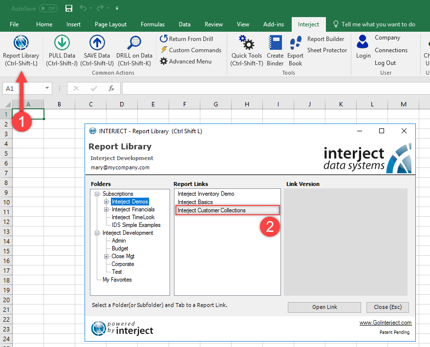
Step 1: In this exercise, you will use the Customer Collections Demo from a previous walkthrough. This demo can be found in the Report Library under the Interject Demo folder as shown below.

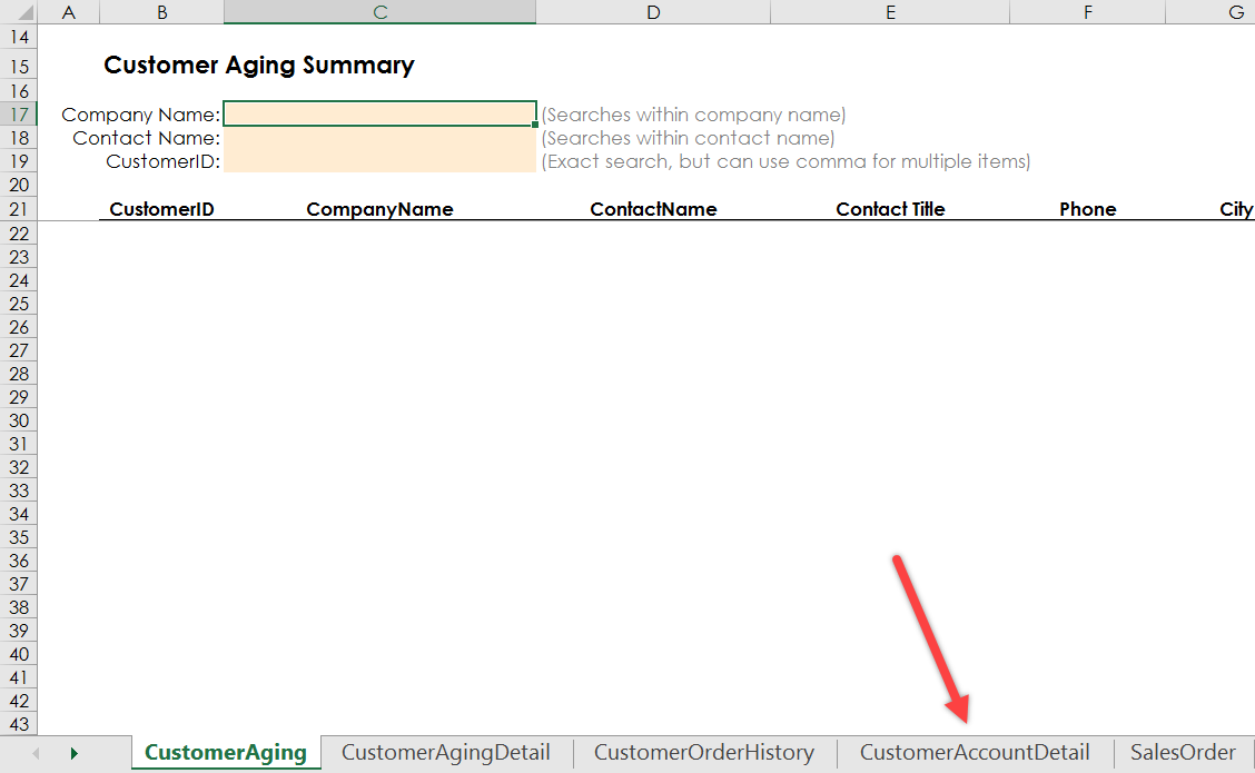
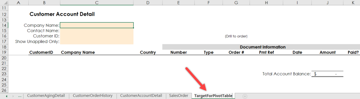
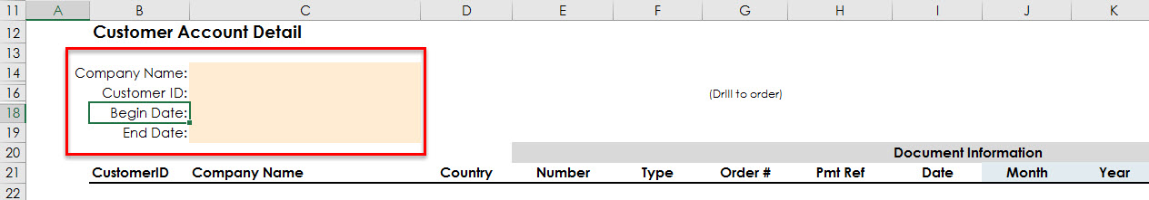
Step 2: When you open the report it will look like the screenshot below. Select the CustomerAccountDetail tab.

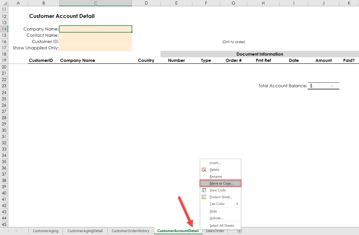
Step 3: To build the Pivot table, right click the CustomerAccountDetail tab and make another copy so you can complete the following steps.

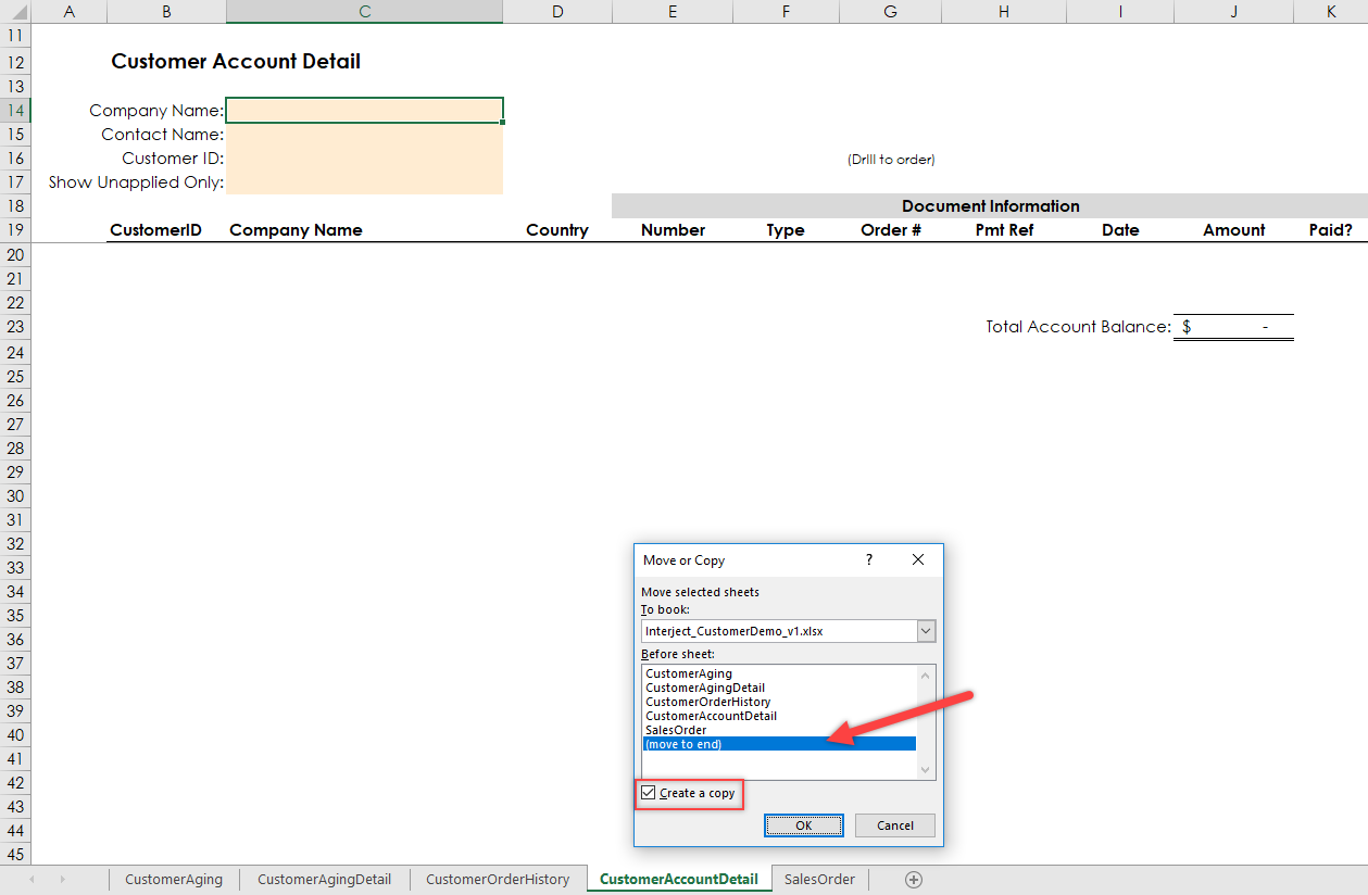
Step 4: In the copy sheet dialog box, select move to end to make the copy at the end of the list of tabs.

Now rename the tab something that represents the data, such as TargetForPivotTable.

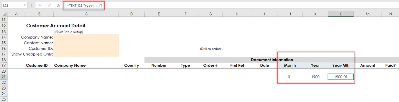
Step 5: Once the tab is copied, you are going to insert 3 columns, separating the date column (column I) into Month, Year, and Year-Mth columns.

In the Month column in cell J21, type =TEXT(I21,"mm").

In the Year column in K21, type =TEXT($I21,"yyyy").

In the Year-Mth column in L21, type =TEXT(I21,"yyyy-mm").

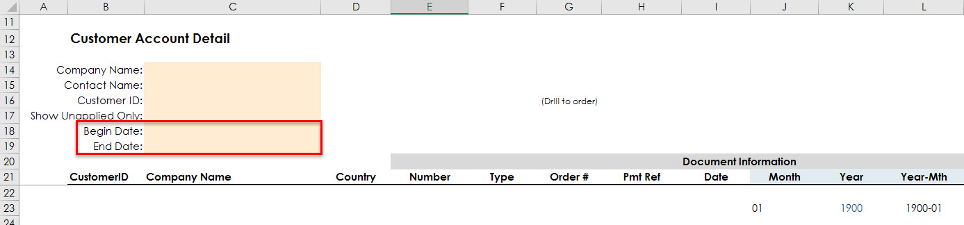
Step 6: Next, you are going to add two parameters to the report by inserting two rows below Show Unapplied Only and labeling them Begin Date: and End Date:.

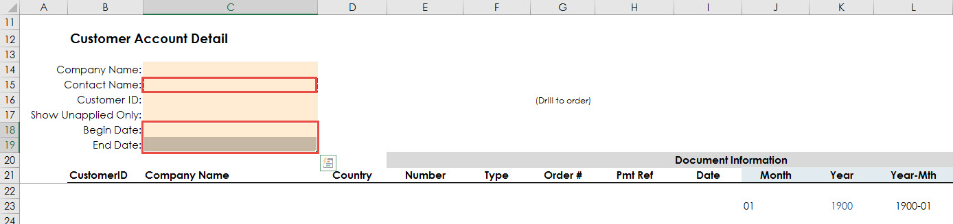
Step 7: Select cell C14 and copy it to C18 and C19.

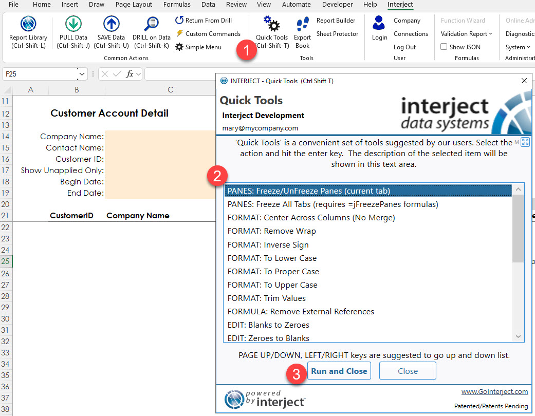
Step 8: Use the quick tools menu in the interject ribbon. In the dialog box select Freeze/UnFreeze Panes (current tab) and click Run and Close.

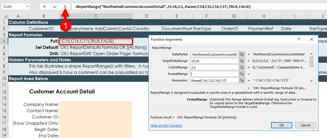
Step 9: Select the report formula in cell C4, then select the function wizard.

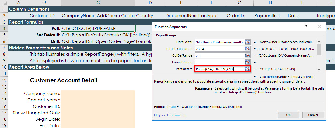
Step 10: In the parameters section of the dialog box change the Parameters field to this: Param(C14,,C16,,C18,C19).

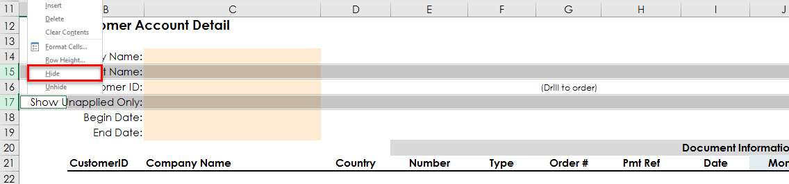
Step 11: Hide rows C15, and C17 since they will not be needed for this report but exist as possible parameters in the stored procedure.

Note: The parameter section of the report should look like the following screenshot.

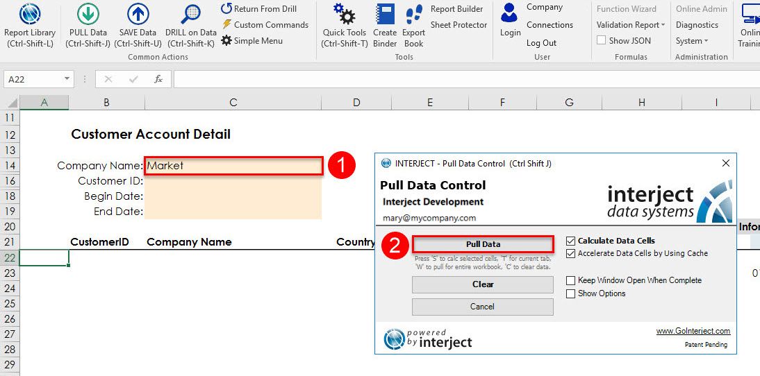
Step 12: Now that you have entered the fields, you can use Pull Data on the report, filtering for companies with Market in their names. First type Market in the filter cell C1 and then Pull Data.

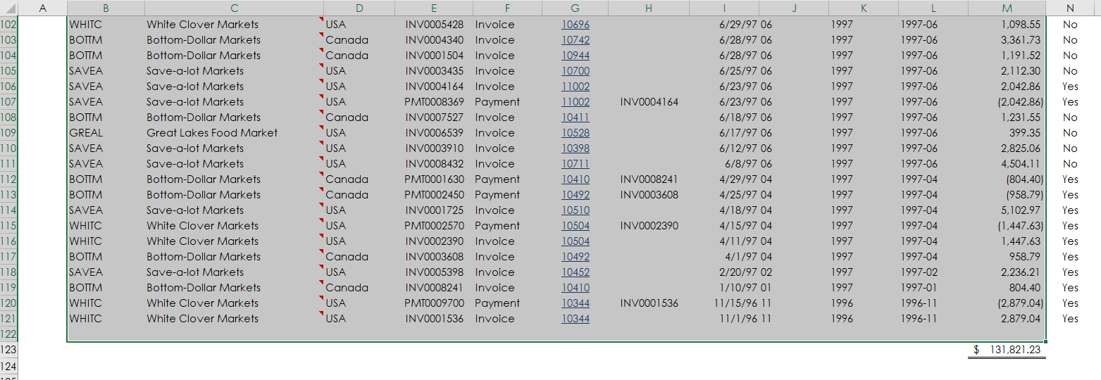
Step 13: Highlight the cells B21 to M122. Important: Be sure to include row 21, the column labels on the top of the range, and include the bottom anchor row, which is one row past the last customer record. The anchor row is important since it will grow and shrink as the data is pulled and cleared. Exclude the Paid? column from the table range.

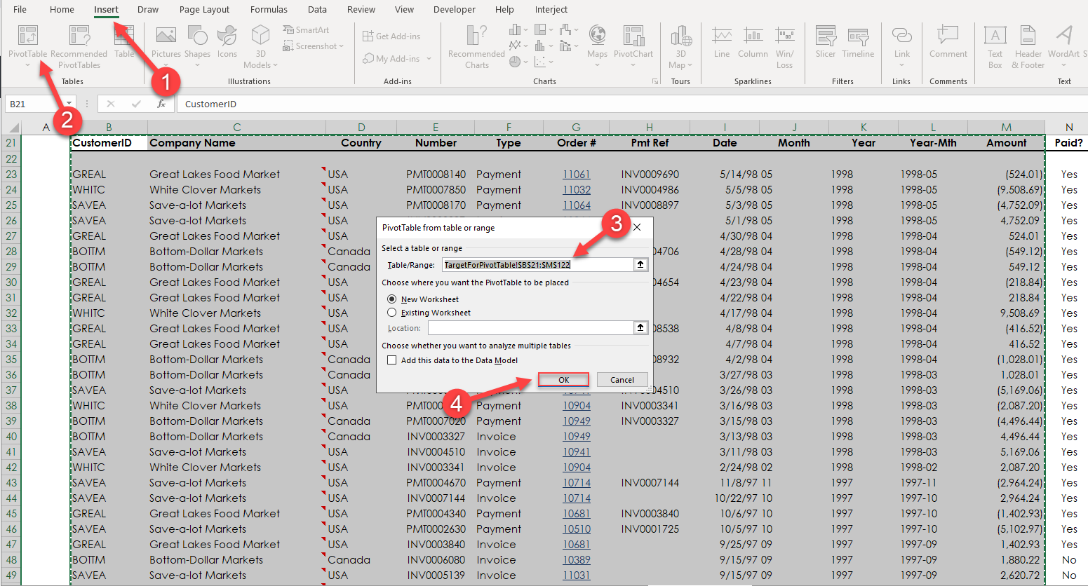
Step 14: In the screenshot below, you can see there are four steps to preparing the contents of the pivot table.

1. Select the Insert ribbon as noted below.
2. Within the Insert ribbon, click the PivotTable menu item so the Create PivotTable window appears.
3. Ensure the range TargetForPivotTable!$B$21:$M$122 is selected in the Select a table or range box.
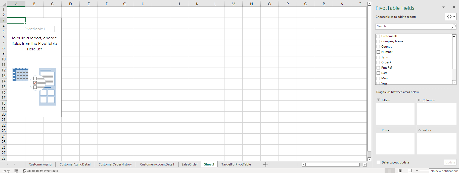
4. Click the OK button, and a new tab will be created with the new pivot table.

Building the Pivot Table

Step 1: From here you can pivot in any way needed.

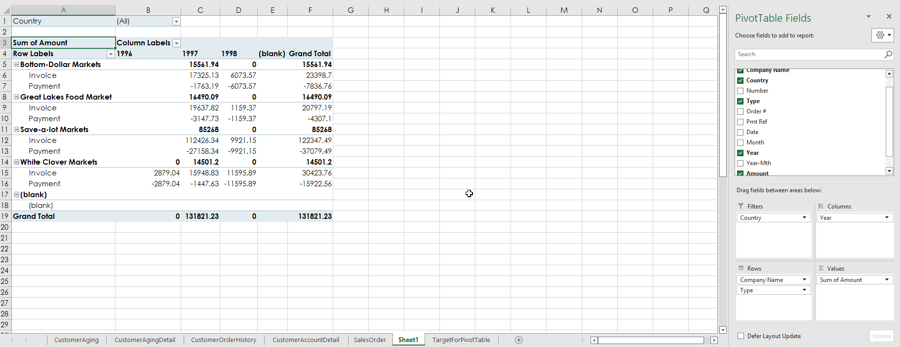
Step 2: Use the PivotTable pane on the right to place Year in the columns. Company Name and Type go to rows, Country goes in Filters. Then, choose the Amount to be summed. Your pivot table should match the screenshot below.

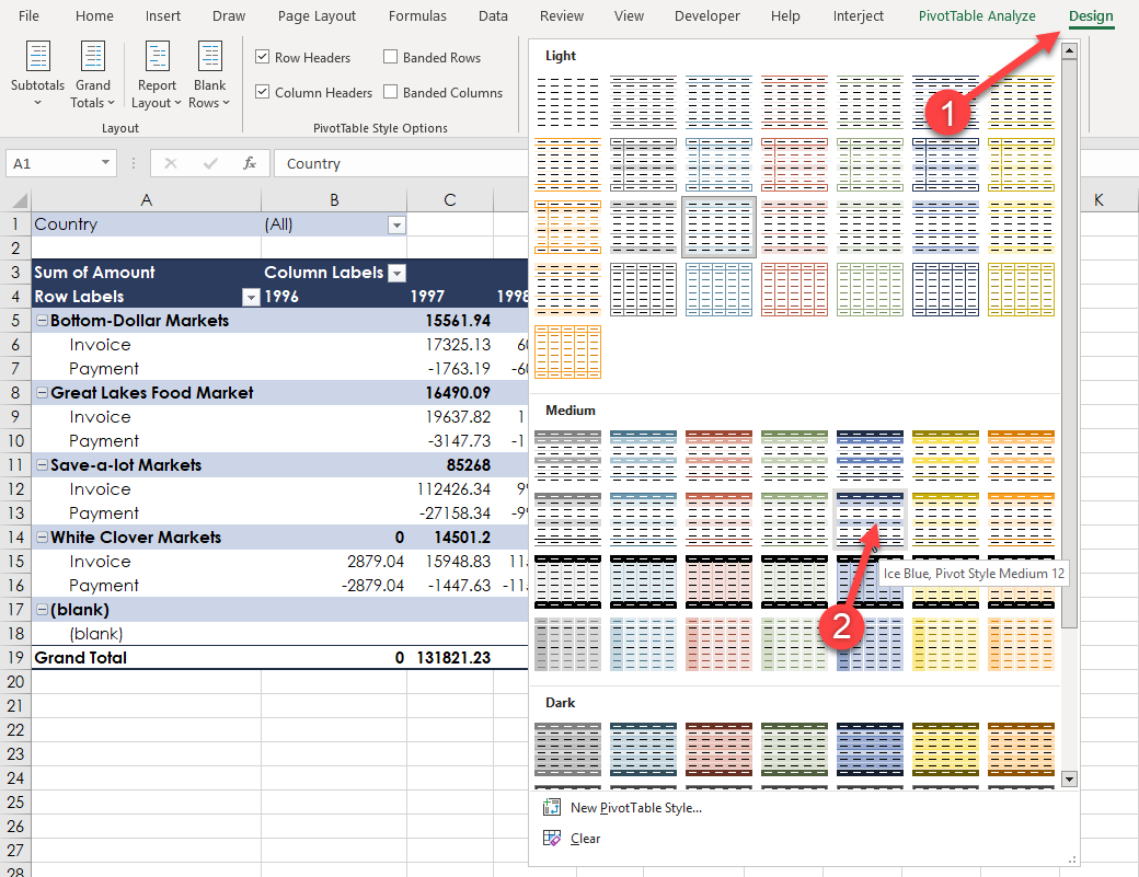
Step 3: Rename the tab "Pivot" and you can customize the look by clicking Design and then expand the table previews and select a color theme.

Customizing the Pivot Table

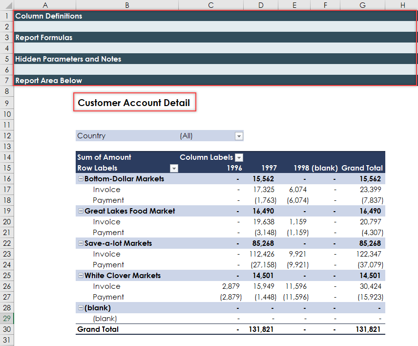
Step 1: Prepare the pivot table worksheet to interact with the Interject worksheet. That way the data can be updated based on select filters, and security can be considered. You will insert the configuration rows at the top as you normally do with Interject reports, but Report Formulas is the only section being used. You will also add a Title and hide the grids.

Step 2: Now set up the ReportRun() function. This will cause the target sheet to perform a Pull Data or Clear Data when Pull Data is triggered from the pivot table worksheet.

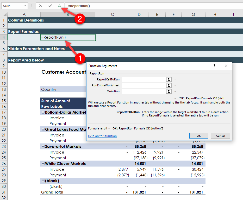
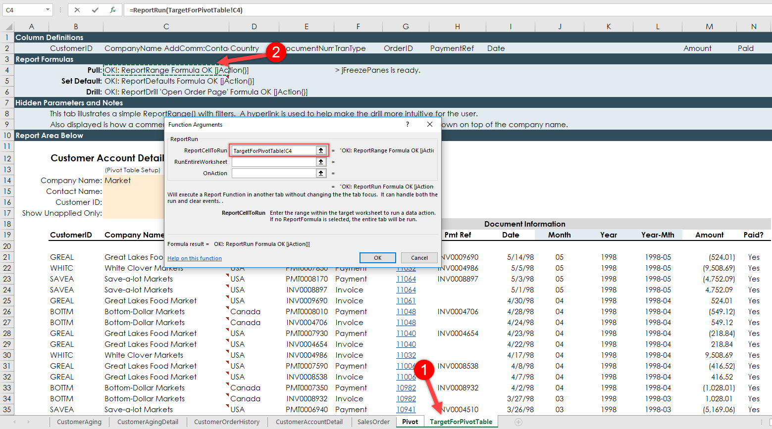
Step 3: In the ReportCellToRun argument, select the TargetForPivotTable tab and select the ReportRange() formula in C4.

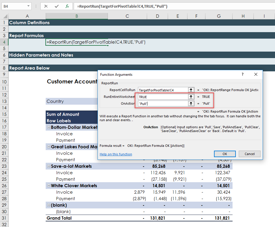
Step 4: Type True in the RunEntireWorksheet argument. And type Pull in the OnAction argument. This will trigger the second worksheet to run only when Pull Data is performed on the current pivot table worksheet.

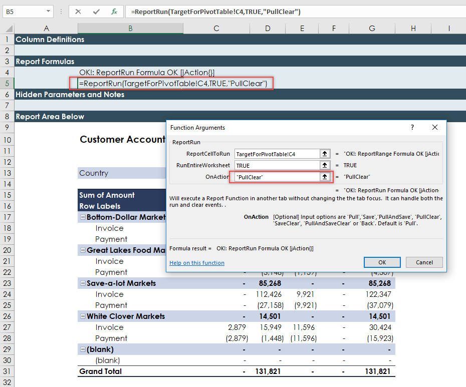
On a second line under row 4 (insert new row if needed), you will do the same for the second ReportRun(). This time, however, type PullClear in the OnAction argument so that the pivot table clear function works correctly.

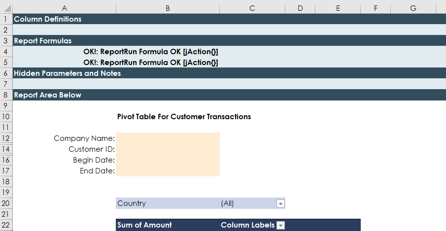
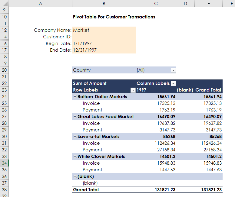
Step 5: Now that the ReportRange() fields are prepared, you can add filters for the searches. Rename the title to Pivot Table For Customer Transactions as seen below. Also, add the filters Company Name, Contact Name, CustomerID, Show Unapplied Only, Begin Date, and End Date. The filters in the Pivot tab should match the filters in the TargetForPivotTable tab.

Note: Remember there are 2 hidden rows that you have to match.

Step 6: Navigate to cell C14 of the TargetForPivotTable tab. Ensure the type is General.

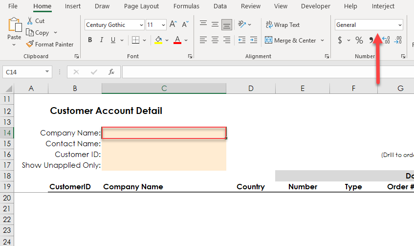
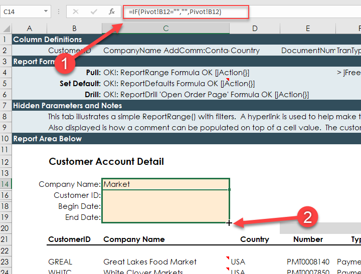
Step 7: For the Company Name, type =if(Pivot!B12="","",Pivot!B12). This formula will make the filters equal between pages and if the Pivot worksheet filter is blank, it will be blank as well. Normally, Excel will make the result 0 if not handled with this formula. Copy cell C14 and paste it through C19 so the other filters are linked as well.

Step 8: Now go back to the pivot table and make sure it is working properly. Enter the following filters to check the pull.

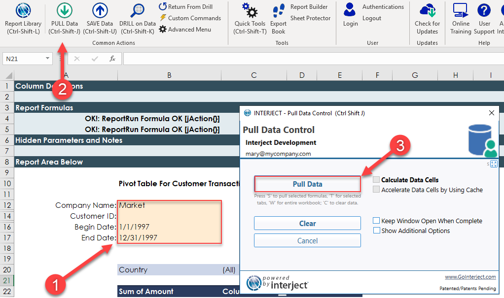
Now you can see that the table only pulled data from transactions occurring in 1997, so the filters, ReportRun(), and pivot table are working as they should.

For more ways to work with a pivot table, see the pivot table section on the customer aging walkthrough.